Markov chain theory
다음 Stochastic process에 대해 생각해보자. $\theta^{(t)} = i$ 라는 표기는 time $t$에 상태 $i$에 있다고 이해하면 된다.
\[{\theta^{(t)},\;\;t=1,2,\cdots}\]우리는 다음 조건을 만족하는 Stochastic process $\theta^{(t)}$를 Markov chain이라고 하다.
\[p(\theta^{(t+1)} \vert \theta^{(1)},\theta^{(2)},\theta^{(3)},\cdots,\theta^{(t)}) = p(\theta^{(t+1)} \vert \theta^{(t)})\]즉, 시점 t+1에서의 상태는 그 직전 시점인 t에서의 상태에만 영향을 받는 것을 뜻한다.
참고로 Transition probability from $i$ to $j$, 즉 $P_{ij}$는 다음 확률을 뜻한다.
\[P_{ij} = P(\theta^{(t+1)}=j \vert \theta^{(t)}=i)\]
MCMC : Markov Chain Monte Carlo
산업공학 등 전통적인 Markov chain과 관련된 분석에서는 Transition Rule: $P(\theta^{(t+1)} \vert \theta^{(t)})$이 주어졌을 때 Stationary Distribution $\pi(\theta)$를 찾는 것에 포커스를 둔다.
반면, 우리는 Target Distribution(Stationary distribution)이 주어졌을 때 efficient한 transition rule을 찾는 것에 큰 관심을 두고자 한다.
Metropolis Algorithm
Metropolis 알고리즘은 MCMC의 초석이 되는 알고리즘이다. 우리는 target distribution $\pi(\theta)$에서 sampling을 하고자 한다. Metropolis Algorithm의 경우 다음의 step을 거쳐 iterative하게 sampling하게 된다.
-
현재 시점은 $t$시점이다. 현재 시점에서의 $\theta^{(t)}$를 given으로 transition kernel $T(\theta^{ * } \vert \theta^{ (t) })$에서 새로운 sample $\theta^{ * }$을 sampling한다.
-
$\alpha = {\pi(\theta^{ * }) \over \pi(\theta^{ (t) })}$ 를 계산한다.
-
$p = min(\alpha, 1)$을 계산한다.
-
다음과 같이 $\theta^{ (t+1) }$을 update한다. \(\begin{align*} \theta^{ (t+1) } = \begin{cases} \theta^{ * }\;\;\;\;with\;prob\;p=min(\alpha,1)\\ \theta^{ (t) }\;\;\;with\;prob\;(1-p) \end{cases} \end{align*}\)
이 과정을 일정 iteration을 반복하여 sampling한다.
단, Metropolis 알고리즘의 경우 Symmetric kernel의 경우에만 한정되어 사용할 수 있다.
Symmetric kernel: $T(\theta^{ * } \vert \theta^{ (t) }) = T(\theta^{ (t) } \vert \theta^{ * }) $
Metropolis Hastings Algorithm
만약 Transition Kernel이 Symmetric하지 않은 경우에는 어떻게 할까? Metropolis 알고리즘을 Non-Symmetric Transition Kernel case로 확장시킨 알고리즘이 바로 Metropolis Hastings 알고리즘이다.
Sampling 과정은 다음과 같다.
-
현재 시점은 t-step이다. 현재 시점에서의 $\theta^{(t)}$를 given으로 transition kernel $T(\theta^{ * } \vert \theta^{ (t) })$에서 새로운 sample $\theta^{ * }$을 sampling한다.
-
$\alpha = {\pi(\theta^{ * })/T(\theta^{ * } \vert \theta^{ (t) }) \over \pi(\theta^{ (t) })/T(\theta^{ (t) } \vert \theta^{ * })}$ 를 계산한다.
-
$p = min(\alpha, 1)$을 계산한다.
-
다음과 같이 $\theta^{ (t+1) }$을 update한다. \(\begin{align*} \theta^{ (t+1) } = \begin{cases} \theta^{ * }\;\;\;\;with\;prob\;p=min(\alpha,1)\\ \theta^{ (t) }\;\;\;with\;prob\;(1-p) \end{cases} \end{align*}\)
단순히 글로만 보면 이해하기가 쉽지 않다. 다음 예시를 통해 Metropolis Hastings Algorithm을 이해해보자.
Example
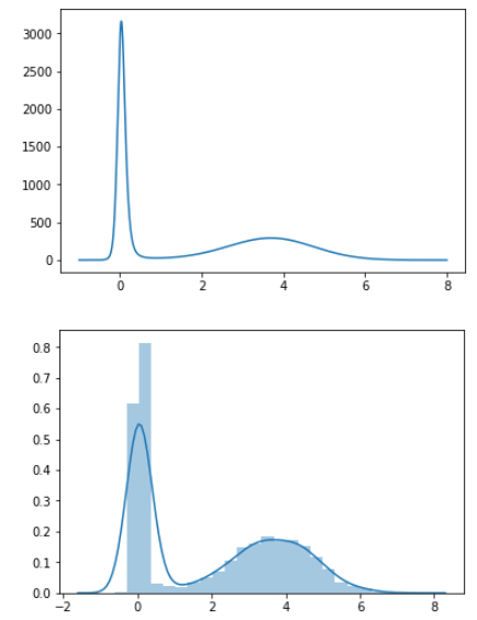
\[Target\;distribution: \pi(x) \propto {1 \over \sqrt{8x^2+1}}exp \left \lbrack -{1 \over 2}(x^2-8x-{16 \over 8x^2+1}) \right \rbrack\] \[Transition\;kernel:T(x' \vert x)=0.6N(x-1.5,1)+0.4N(x+1.5,1)\]10000번의 iteration을 통하여 Metropolis Hastings 알고리즘으로 $x$를 sampling하는 과정은 다음과 같다.
import numpy as np
import scipy.stats as stats

def target_fn(x):
    density = 1/(np.sqrt(8*(x**2)+1))*np.exp(-0.5*(x**2-8*x-16/(8*(x**2)+1)))
    return density

def transition_kernel(x,mu):
    d1 = 0.6*stats.norm.pdf(x,loc=mu-1.5,scale=1) #mu, sigma, size
    d2 = 0.4*stats.norm.pdf(x,loc=mu+1.5,scale=1) #mu, sigma, size
    trans = d1+d2
    return trans

n_iter = 10000
n_accept = 0
x = np.zeros(n_iter+1)
x[0] = 1 #starting point

for t in range(n_iter):
    x_t = x[t]

    z = np.random.binomial(1,0.6,1)
    if z==1:
        x_prime = np.random.normal(x_t-1.5,1,1)
    else:
        x_prime = np.random.normal(x_t+1.5,1,1)

    alpha = (target_fn(x_prime)/transition_kernel(x_prime,x_t)) / (target_fn(x_t)/transition_kernel(x_t,x_prime))

    runif = np.random.uniform(0,1,1)
    if runif <= alpha:
        x[t+1] = x_prime
        n_accept += 1
    else:
        x[t+1] = x[t]
그 결과, target distribution(윗쪽 그림)과 거의 동일하게 sampling된 것(아래쪽 그림)을 확인할 수 있다.
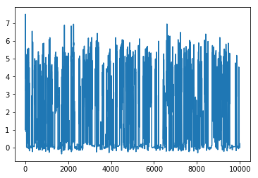
Time series plot이라고도 불리우는 Trace plot을 그려보았을 때에도 다음과 같이 잘 수렴하고 있는 것을 확인할 수 있다.