Estimating pdf $f$
앞선 포스트에서 EDF를 통해 cdf $F$를 간단하게 추정하는 방법에 대해 살펴보았다. 이번 포스트에서는 Histogram Estimate/Naive Density Estimate/Kernel Density Estimate를 통하여 pdf $f$를 Estimate하는 방법에 대해 살펴보도록 하겠다.
1. Histogram Estimate
Histogram estimate는 말 그대로 histogram을 통하여 pdf $f$를 estimate하는 방법이다. Histogram estimate는 다음 3가지 특성을 가진다.
-
locations 와 widths of the bins 에 큰 영향을 받는다.
-
locations 와 widths of the bins 가 적절하게 선택이 잘 된다면, performance가 꽤 좋다.
-
Blocky하고, discontinuous하다.
Example: Yellowstone National Park dataset
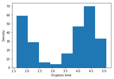
bins = 8일 때의 histogram이다.
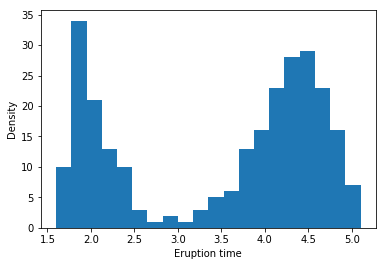
bins = 20일 때의 histogram이다.
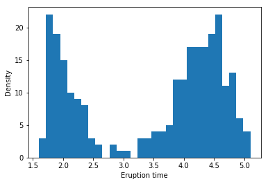
bins = 30일 때의 histogram이다.
2. Naive Density Estimate
pdf $f$를 추정하는 또 다른 방법으로 Empirical Density Estimate를 확장시킨 Naive Density Estimate가 있다. 우리는 다음과 같이 cdf $F$에 대한 derivative로 pdf $f$를 구할 수 있다는 사실을 알고 있다.
\[f(x) = \lim_{h \to 0} {F(x+h)-F(x-h) \over 2h}\]이 사실을 활용하여 h를 아주 작은 어떠한 값으로 정한다면 우리는 Empirical Density Estimate $\hat {F(x)}$를 활용하여 다음과 같이 $f(x)$를 $\hat {f(x)}$로 추정할 수 있다.
\[\begin{align*} \hat f(x) &\equiv {1 \over {2h}} \left( \hat F_n(x+h) - \hat F_n(x-h) \right)\\ & = {1 \over {2nh}} \left( \sum_{j=1}^n I(x-h < x_j \leq x+h) \right)\\ & = {1 \over n} \left( \sum_{j=1}^n {1 \over h} {1 \over 2} I(-1 < {x-x_j \over h} \leq 1) \right)\\ & = {1 \over n} \left( \sum_{j=1}^n {1 \over h} K({x-x_j \over h}) \right)\\ where\;\;K(x)&= { 1 \over 2 } \cdot I(-1 < x \leq 1) \end{align*}\]
Naive Density Estimator Souce code
def indicator(x):
    if -1<x<=1:
        result = 1
    else:
        result = 0

    return result

def K(x):
    result = 1/2*indicator(x)

    return result

def naive_density_estimate(x, h, data):
    n = len(data)
    summation = []
    for i in range(n):
        summation.append(K((x-data[i])/h)/h)
    result = 1/n*sum(summation)

    return result
Example: Yellowstone National Park dataset
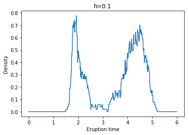

각각 왼쪽 위부터 h = 0.1, 0.2, 0.3, 0.4, 0.5, 0.6일 때 Naive Density Estimate의 결과이다.
우리가 이 예시를 통해 확인할 수 있는 Naive Density Estimate의 단점이 있는데, 위 결과에서 볼 수 있듯이 추정된 pdf가 continuous하지 않으며, 상당히 ragged되어 있다는 것이다.(The naive density estimator is not continuous and will have a ragged pattern.)
3. Kernel Density Estimator: KDE
앞서 Naive Density Estimate를 다음과 같이 할 수 있다는 것을 살펴보았다.
\[\begin{align*} \hat f(x) & = {1 \over n} \left( \sum_{j=1}^n {1 \over h} K({x-x_j \over h}) \right)\\ \end{align*}\]Naive Density Estimator에서는 $K(x)$ function을 $K(x) = { 1 \over 2 } \cdot I(-1 < x \leq 1)$로 잡고 $ \hat f(x) $를 구했다. 이 $K(x)$를 자세히 살펴보면 Uniform(-1,1) 분포에 해당하는 Kernel이라는 사실을 알 수 있다.
이 Kernel function을 어떠한 분포의 kernel로 바꾸느냐에 따라 또다른 Estimator가 될 수 있다. Naive Density Estimator에서 Uniform Kernel이 아닌 다른 분포의 Kernel을 사용할 때 우리는 이를 Kernel Density Estimator, KDE라고 한다.
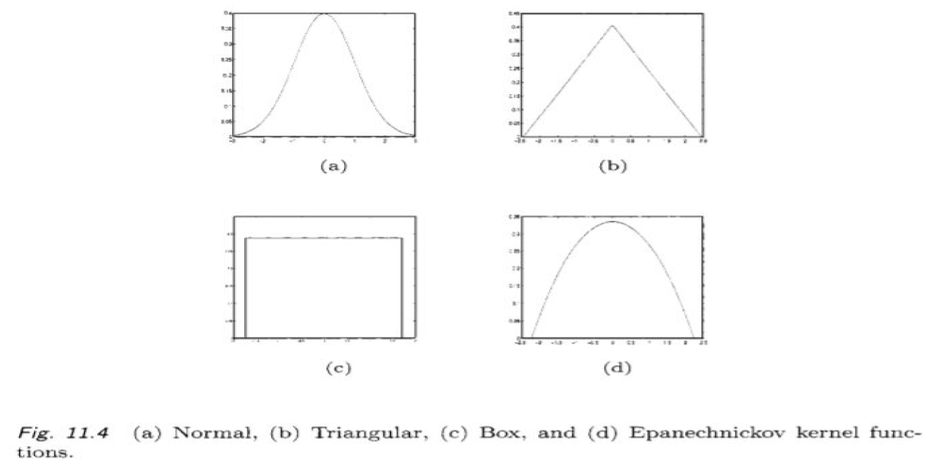
Gaussian density와 같이 smooth한 kernel function을 사용할 경우, Naive Density Estimator와는 다르게 smooth한 $\hat f$를 얻을 수 있다. Gaussian Kernel(Normal Kernel) 이외에도 Triangular, Box, Epanechnickov kernel 등을 사용할 수 있다.
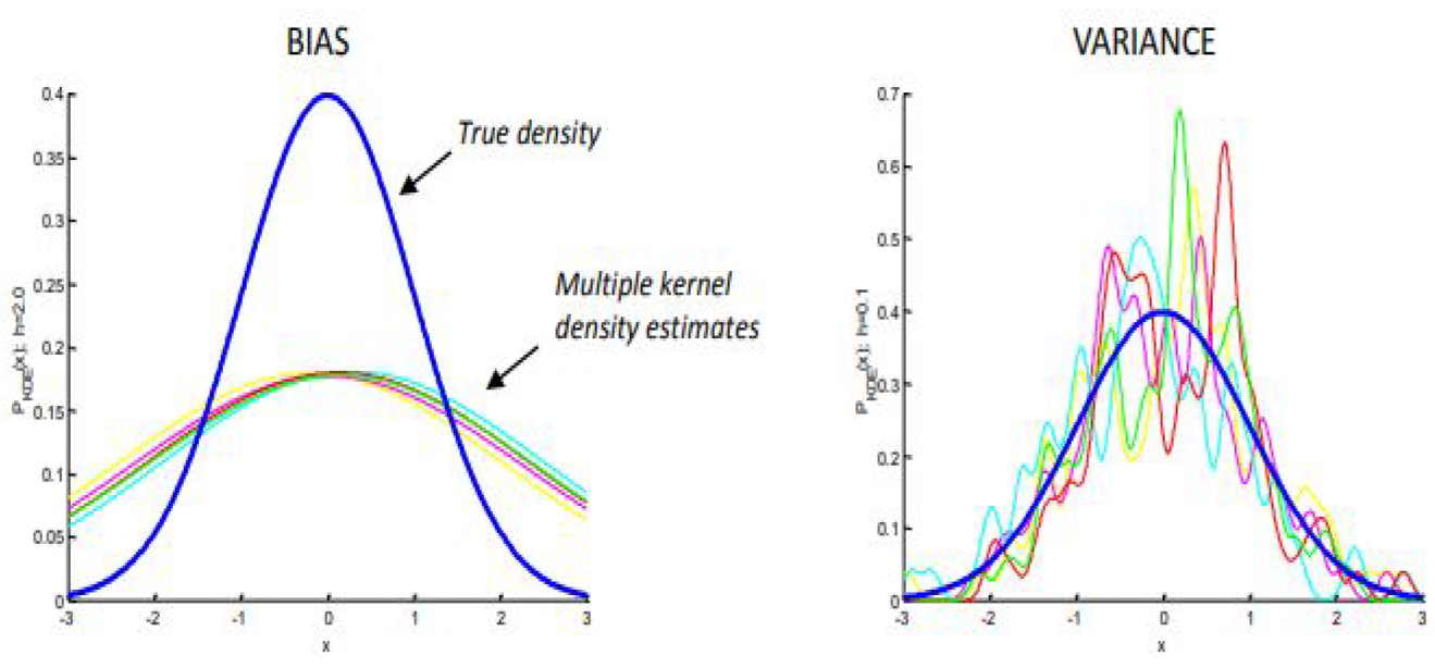
KDE는 Kernel의 선택 뿐만아니라, h(Bandwidth)의 선택 또한 중요하다. h의 선택에 따라 bias와 variance는 trade-off 관계에 있는데, h가 커질수록($h \rightarrow \infty$) Bias가 증가하고 Variance가 줄어든다. 반면, h가 작아질수록($h \rightarrow 0$) Bias가 감소하고 Variance가 증가하게 된다.
KDE Souce code
import scipy.stats as stats

def K(x):
    result = stats.norm.pdf(x,loc=0,scale=1)

    return result

def KDE(x, h, data):
    n = len(data)
    summation = []
    for i in range(n):
        summation.append(K((x-data[i])/h)/h)
    result = 1/n*sum(summation)

    return result
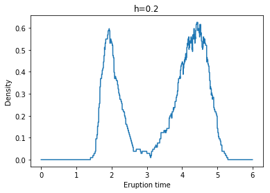
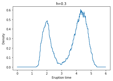
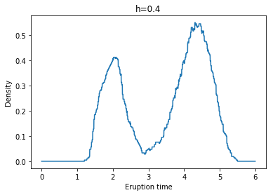
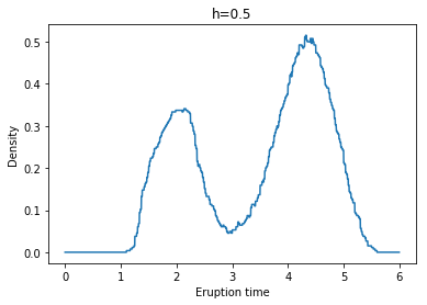
Example: Yellowstone National Park dataset
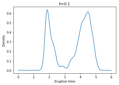
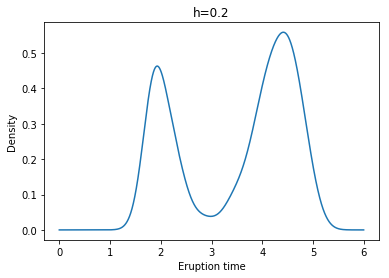
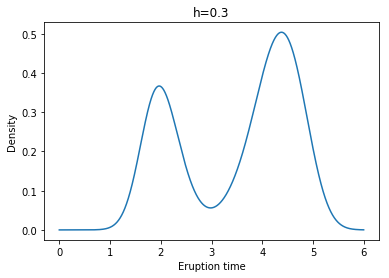
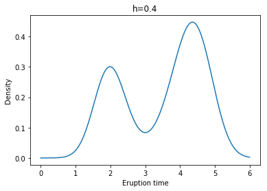
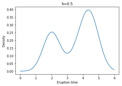
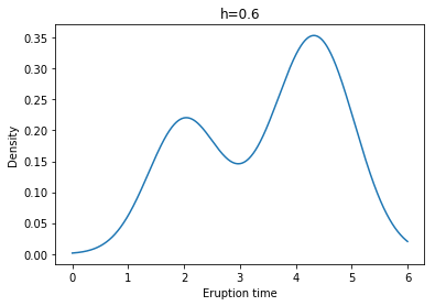
각각 왼쪽 위부터 h = 0.1, 0.2, 0.3, 0.4, 0.5, 0.6일 때 Kernel Density Estimate(with Gaussian Kernel)의 결과이다.
Reference
Sangun Park(2019), Nonparametric Statistics: Nonparametric Density Estimation, Yonsei University