Multiple Linear Regression

우선, 해당 포스트는 Stanford University School of Engineering의 CS231n 강의자료와 모두를 위한 딥러닝 시즌2의 자료를 기본으로 하여 정리한 내용임을 밝힙니다.

Multiple linear regression

이번 포스트에서는 Multivariate Multiple linear regression에 대해 살펴볼 것이다.

이에 앞서, 우리는 Linear Regression 포스트에서 Simple linear regression에 대해 살펴보았다. Simple linear regression은 하나의 $y$와 하나의 $x$간의 선형관계에 대한 이야기였다.

Multiple linear regression의 경우, 하나의 $y$와 여러 $x_i(i=1,2,\cdots,p)$들 사이의 선형관계에 대한 이야기다. 따라서 모형은 다음과 같다.

\[H(x_1, x_2, x_3) = x_1w_1 + x_2w_2 + x_3w_3 + b\] \[cost(W, b) = \frac{1}{n} \sum^n_{i=1} \left( H(x^{(i)}) - y^{(i)} \right)^2\]

Multiple linear regression

따라서 Multiple linear regression 모형을 행렬로 나타내면 다음과 같다.

\[\begin{align*} H(X) &= XW\\ &= \begin{pmatrix} 1 & X_1 & X_2 & X_3 \end{pmatrix} \cdot \begin{pmatrix} b\\ w_1 \\ w_2 \\ w_3 \\ \end{pmatrix}\\ &= b+ X_1w_1 + X_2w_2 + X_3w_3 \end{align*}\]

Example

학생 5명의 First Quiz/Second Quiz/Third Quiz 점수와 기말고사 성적(Final score)에 대하여 다음과 같은 data를 가지고 있다고 가정하자.

A학생의 경우 퀴즈 성적은 73, 80, 75였으며, 기말고사 성적은 152점이었다. B학생의 경우 퀴즈 성적은 93, 88, 93였으며, 기말고사 성적은 185점이었다. C학생의 경우 퀴즈 성적은 89, 91, 90였으며, 기말고사 성적은 180점이었다. D학생의 경우 퀴즈 성적은 96, 98, 100였으며, 기말고사 성적은 196점이었다. E학생의 경우 퀴즈 성적은 73, 66, 70였으며, 기말고사 성적은 142점이었다.

우리는 First/Second/Third 퀴즈의 점수($X$)와 기말고사 성적$Y$간의 관계에 대해 regression 모형을 세우려고 한다.

이 regression 모형의 weights에 대한 optimization 과정은 다음과 같다. Hypothesis를 정의하는 부분을 제외하면 Simple linear regression의 문제를 푸는 code와 거의 완벽하게 같다. 자세한 설명은 Linear Regression에서 하였으니 참고하면 된다.

import torch

# dataset
x_train = torch.FloatTensor([[73, 80, 75],
                             [93, 88, 93],
                             [89, 91, 90],
                             [96, 98, 100],
                             [73, 66, 70]])
y_train = torch.FloatTensor([[152], [185], [180], [196], [142]])

print(x_train.shape)
print(y_train.shape)

# weight initialization
W = torch.zeros((3, 1), requires_grad=True)
b = torch.zeros(1, requires_grad=True)

# optimizer
optimizer = torch.optim.SGD([W, b], lr=1e-5)

n_epochs = 20
for epoch in range(n_epochs + 1):
    # H(x)
    hypothesis = x_train.matmul(W) + b

    # cost
    cost = torch.mean((hypothesis - y_train) ** 2)

    # updating weights
    optimizer.zero_grad()
    cost.backward()
    optimizer.step()

    # print
    print('Epoch {:4d}/{} hypothesis: {} Cost: {:.6f}'.format(
        epoch, n_epochs, hypothesis.squeeze().detach(), cost.item()
    ))

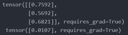
최종 iteration에서의 weights를 확인해보면 위와 같다. 즉 우리는 최종적으로 다음과 같은 Regression 모형을 세우게 된 것이다.

\[y = 0.7592x_1 + 0.5692x_2 + 0.6821x_3 + 0.0107\]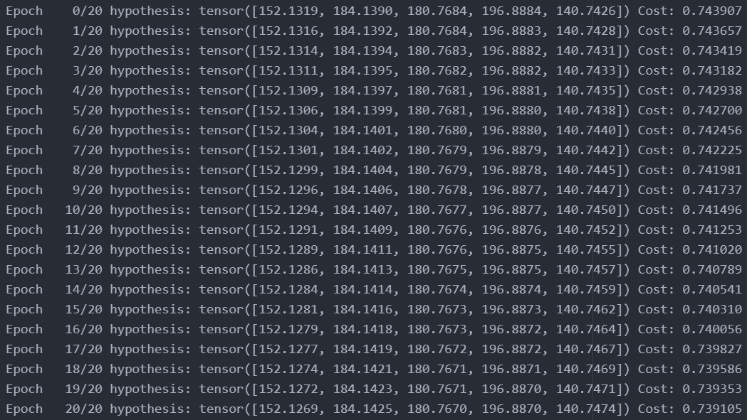

최종 iteration에서의 weights로 구한 Hypothesis 값들은 $\hat y_1 = 152.1269$, $\hat y_2 = 184.1425$, $\hat y_3 = 180.7670$, $\hat y_4 = 196.8870$, $\hat y_5 = 140.7474$로써 실제 $y$값들과 거의 같은 것을 확인할 수 있다.

High level API

사실 linear regression과 같이 아주 간단한 모형의 경우 hypothesis = x_train.matmul(W) + b, cost = torch.mean((hypothesis - y_train) ** 2)과 같이 일일이 계산하는 과정을 명시해줄 수 있다. 하지만 Deep learning과 같이 모형이 조금만 더 복잡해지더라도 이러한 작업은 매우 힘들며, 거의 불가능해 진다.

다행히 Pytorch는 이러한 작업을 쉽게 할 수 있는 High-level API를 제공한다. 아래 예시에서는 torch.nn.Module, torch.nn.Linear(), torch.nn.functional.mse_loss()등의 함수를 사용하여 계산 과정을 일일이 명시하지 않고도 linear regression 모형을 만들게 수 있게 된다.

Source code

import torch

class LinearRegressionModel(torch.nn.Module):
    def __init__(self):
        super().__init__()
        self.linear = torch.nn.Linear(1, 1)

    def forward(self, x):
        return self.linear(x)

class MultivariateLinearRegressionModel(torch.nn.Module):
    def __init__(self):
        super().__init__()
        self.linear = torch.nn.Linear(3, 1)

    def forward(self, x):
        return self.linear(x)

# dataset
x_train = torch.FloatTensor([[73, 80, 75],
                             [93, 88, 93],
                             [89, 91, 90],
                             [96, 98, 100],
                             [73, 66, 70]])
y_train = torch.FloatTensor([[152], [185], [180], [196], [142]])

# weight initialization
model = MultivariateLinearRegressionModel()

# optimizer
optimizer = torch.optim.SGD(model.parameters(), lr=1e-5)

n_epochs = 20
for epoch in range(n_epochs+1):
    # H(x)
    prediction = model(x_train)

    # cost
    cost = torch.nn.functional.mse_loss(prediction, y_train)

    # updating weights
    optimizer.zero_grad()
    cost.backward()
    optimizer.step()

    # print
    print('Epoch {:4d}/{} Cost: {:.6f}'.format(
        epoch, n_epochs, cost.item()
    ))

Reference

CS231n, Stanford University School of Engineering

모두를 위한 딥러닝 시즌2