Softmax Classifier(3) with MNIST

우선, 해당 포스트는 Stanford University School of Engineering의 CS231n 강의자료와 모두를 위한 딥러닝 시즌2의 자료를 기본으로 하여 정리한 내용임을 밝힙니다.

Image Data

이전 포스트에서 정형데이터(Structured Data)에 대한 분류 문제를 Softmax Classifier(Multiclass Logistic Regression)을 통해 풀어보고, Pytorch로 구현해 보았다.

이번 포스트에서는 비정형데이터(Unstructured Data) 중 이미지 데이터(Image data)의 분류 문제를 풀어보도록 하겠다.

MNIST Dataset

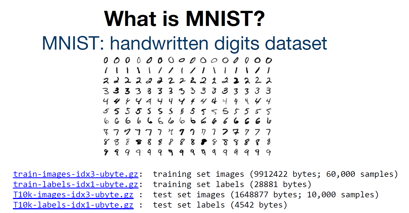
MNIST 데이터셋은 손으로 쓴 숫자 이미지로 이루어진 대형 데이터셋이며, 60,000개의 Training dataset과 10,000개의 Test dataset으로 이루어져 있다.

MNIST 데이터셋(Modified National Institute of Standards and Technology database)은 NIST의 오리지널 데이터셋의 샘플을 재가공하여 만들어졌다. MNIST의 Training set의 절반과 Test set의 절반은 NIST의 Training set에서 취합하였으며, 그 밖의 Training set의 절반과 Test set의 절반은 NIST의 Test set으로부터 취합되었다.

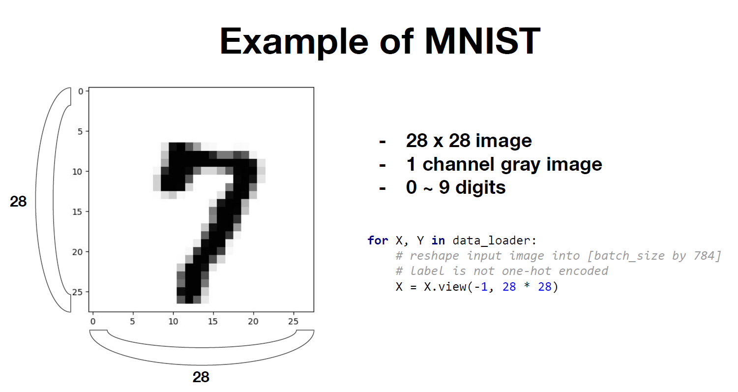
각 데이터는 0에서 9까지의 자연수 중 하나에 대응되는 숫자에 대한 데이터이며, $1 \times 28 \times 28$, 총 784개의 픽셀의 색에 대한 정보를 담은 행렬이다. 각 픽셀에 대응되는 행렬의 성분은 0부터 255사이의 숫자를 가지고 있는데, 까만색에 가까운 픽셀일수록 0에 가까운 값을, 흰색에 가까운 픽셀일수록 255에 가까운 값을 가지게 된다.

Show images of the MNIST

import matplotlib.pyplot as plt
import random
import torch
import torchvision
import torchvision.transforms as transforms

# MNIST dataset
mnist_train = torchvision.datasets.MNIST(root='MNIST_data/',
                          train=True,
                          transform=transforms.ToTensor(),
                          download=True)

mnist_test = torchvision.datasets.MNIST(root='MNIST_data/',
                         train=False,
                         transform=transforms.ToTensor(),
                         download=True)

# parameters
batch_size = 1000

# dataset loader
data_loader = torch.utils.data.DataLoader(dataset=mnist_train,
                                          batch_size=batch_size,
                                          shuffle=True,
                                          drop_last=True)

# show images
idx = range(3)
for i in idx:
    x, y = mnist_train[i][0], mnist_train[i][1]

    plt.title('%i' % y)
    plt.imshow(x.squeeze().numpy(), cmap='gray')
    plt.savefig("image%d"%i)
    plt.show()

한 줄 한 줄씩 살펴보도록 하자. 우선, torchvision.datasets.MNIST()함수를 통하여 torchvision library에 내장되어 있는 MNIST dataset을 읽어온다. train 옵션의 경우 training dataset을 불러오려면 True, test dataset을 불러오려면 False를 사용한다. 이 함수는 결과적으로 (X, Y)과 같이 2개의 원소로 이루어진 tuple을 받아온다. transform 옵션은 이 중 X의 형태에 대한 옵션이다. 이 옵션을 False로 주면 이미지 데이터를 PIL로 받아오기 때문에, Pytorch Tensor로 가져오기 위해서는 True로 설정해주어야 한다. True로 설정해주면 X를 torch.Size([1, 28, 28]) 형태의 Tensor로 가져오게 된다. Y의 경우 transform 옵션의 여부와 상관 없이 0~9사이의 int타입 정수로 가져온다.

MNIST training data의 경우 60,000개의 데이터를 가지고 있는데, 이를 한 번에 불러오는 것은 메모리 문제 때문에 효율적이지 않다. 따라서 mini-batch 단위로 사진을 가지고오는 방법을 선택하게 된다. 적당히 적은 숫자를 사용하면 되는데, 이 예시에서는 1,000개로 선택해 주었다. 그리고 torch.utils.data.DataLoader()를 통하여 설정해준 batch_size 크기 만큼의 데이터를 가져오게 된다. shuffle 옵션의 경우 데이터를 불러들일 때 순서를 섞을 것인지에 대한 옵션이고, drop_last 옵션의 경우 batch 단위로 데이터를 잘라서 읽는 과정에서 데이터의 끝부분이 짤리는 경우가 발생할 때 이를 어떻게 처리할지에 대한 옵션이다.

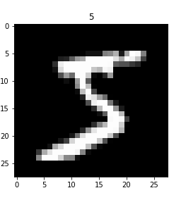
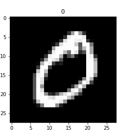
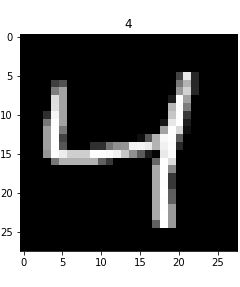
이렇게 가져온 X데이터의 경우 torch.Size([1, 28, 28]) 의 shape을 가진다. x.squeeze()를 통해 X 행렬의 형태를 torch.Size([28, 28]) 으로 reshape해주고, numpy로 변환하여 matplotlib.imshow() 함수를 사용하면 $28 \times 28$의 행렬을 시각적으로 확인할 수 있게 된다.

예시로 0~2의 index에 해당하는 3개의 training 데이터만 시각화 해보면 다음과 같다.

Training Softmax Classifier

Training data $X$의 shape이 $1 \times 28 \times 28$이 되었고, class의 수가 10개인 상태로 문제가 바뀌었지만, 문제를 푸는 방법은 앞서 살펴보았던 정형 데이터에서의 방법과 여전히 같다.

import torch
import torchvision.datasets as dsets
import torchvision.transforms as transforms
import matplotlib.pyplot as plt
import random

# setting device(cpu/gpu)
device = 'cuda' if torch.cuda.is_available() else 'cpu'
print(device)

# for reproducibility
random.seed(777)
torch.manual_seed(777)
if device == 'cuda':
    torch.cuda.manual_seed_all(777)

# parameters
training_epochs = 15
batch_size = 1000

# MNIST dataset
mnist_train = dsets.MNIST(root='MNIST_data/',
                          train=True,
                          transform=transforms.ToTensor(),
                          download=True)

mnist_test = dsets.MNIST(root='MNIST_data/',
                         train=False,
                         transform=transforms.ToTensor(),
                         download=True)

# dataset loader
data_loader = torch.utils.data.DataLoader(dataset=mnist_train,
                                          batch_size=batch_size,
                                          shuffle=True,
                                          drop_last=True)

# MNIST data image of shape 28 * 28 = 784
linear = torch.nn.Linear(784, 10, bias=True).to(device)

# define cost/loss & optimizer
criterion = torch.nn.CrossEntropyLoss().to(device)    # Softmax is internally computed.
optimizer = torch.optim.SGD(linear.parameters(), lr=0.1)

# training
for epoch in range(training_epochs):
    avg_cost = 0
    total_batch = len(data_loader)

    for X, Y in data_loader:
        # reshape input image into [batch_size by 784]
        # label is not one-hot encoded
        X = X.view(-1, 28 * 28).to(device)
        Y = Y.to(device)

        #cost
        hypothesis = linear(X)
        cost = criterion(hypothesis, Y)

        #updating weights
        optimizer.zero_grad()
        cost.backward()
        optimizer.step()

        avg_cost += cost / total_batch

    print('Epoch:', '%04d' % (epoch + 1), 'cost =', '{:.9f}'.format(avg_cost))
print('Learning finished')

중요하다고 생각되는 부분들에 대하여 하나씩 살펴보도록 하자.

# MNIST data image of shape 28 * 28 = 784
linear = torch.nn.Linear(784, 10, bias=True).to(device)

MNIST 데이터셋의 경우 $1 \times 28 \times 28$ 형태의 데이터를 가지고 있다. 우리는 이 $1 \times 28 \times 28$ 데이터를 $1 \times 784$과 같이 일자로 펴진 하나의 벡터 형태로 reshape하여 사용할 것이다.

즉, 우리의 모델은 총 $28 \cdot 28 = 784$개의 weight을 가지게 된다. 또한, 숫자 0부터 9까지 총 10개의 class가 존재하므로, weight matrix의 형태는 $784 \times 10$이 된다. 이를 linear = torch.nn.Linear(784, 10, bias=True).to(device)에 명시해주도록 한다.

# training
for epoch in range(training_epochs):
    avg_cost = 0
    total_batch = len(data_loader)

    for X, Y in data_loader:
        # reshape input image into [batch_size by 784]
        # label is not one-hot encoded
        X = X.view(-1, 28 * 28).to(device)
        Y = Y.to(device)

Training 과정에 대하여 자세히 살펴보도록 하자. 우리는 batch_size를 1000으로 지정해 주었으므로, 한 epoch에서 batch의 총 개수는 60개, iteration 수는 60번이 되는 것이다.

즉 우리의 training 과정은 15번의 Epoch을 거쳐 총 900번의 iteration이 이루어지는 것이다. 한 iteration에서 가져오는 data의 수(batch size)는 1000이므로, training data $X$의 shape은 $1000 \times 784$가 된다. 그러한 이유로 X = X.view(-1, 28 * 28).to(device)에서 X의 shape을 $1000 \times 784$ 로 정해준 것이다.

Test

# Test the model using test sets
with torch.no_grad():
    X_test = mnist_test.data.view(-1, 28 * 28).float().to(device)
    Y_test = mnist_test.targets.to(device)

    prediction = linear(X_test)
    correct_prediction = torch.argmax(prediction, 1) == Y_test
    accuracy = correct_prediction.float().mean()
    print('Accuracy:', accuracy.item())

    # Get one and predict
    r = random.randint(0, len(mnist_test) - 1)
    X_single_data = mnist_test.data[r:r + 1].view(-1, 28 * 28).float().to(device)
    Y_single_data = mnist_test.targets[r:r + 1].to(device)

    print('Label: ', Y_single_data.item())
    single_prediction = linear(X_single_data)
    print('Prediction: ', torch.argmax(single_prediction, 1).item())

    plt.imshow(mnist_test.data[r:r + 1].view(28, 28), cmap='Greys', interpolation='nearest')
    plt.show()

약 Accuracy 86.9%의 성능을 보이는데, 얼핏 생각하면 높은 수치로 보이지만 사실은 훌륭한 성능은 아니다. 우리가 사용한 모델은 $28 \times 28$의 이미지 데이터를 $1 \times 784$ 형태의 vector로 flatten시킨 후 Softmax classifier를 적용한 것인데, 이로 인하여 위치에 대한 정보를 모두 잃어버리게 되어 효율적이지 못한 방법이 되어버린다.

이후에 보게 될 CNN 기반의 모델에서는 전혀 다른 방법을 사용하여 이미지 데이터에 대한 분류 알고리즘을 세우게 되고, MNIST dataset의 classification 문제에 대한 Accuracy를 거의 100%에 가깝께까지 끌어올릴 수 있게 된다.

Reference

CS231n, Stanford University School of Engineering

모두를 위한 딥러닝 시즌2