Multi layer perceptron(MLP)

우선, 해당 포스트는 Stanford University School of Engineering의 CS231n 강의자료와 모두를 위한 딥러닝 시즌2의 자료를 기본으로 하여 정리한 내용임을 밝힙니다.

XOR problem

XOR gate

앞의 포스트에서 XOR gate는 단층 perceptron으로 풀 수 없다는 사실을 확인하였다.

XOR gate가 무엇인지 다시 한 번 살펴보자.

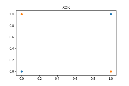
XOR 게이트는 두 개의 입력 값 $x_1$과 $x_2$가 모두 0이거나, 모두 1인 경우에만 출력값 $y$가 0이고, 나머지의 경우에는 1이 나오는 구조를 가지고 있다. 이를 그림으로 나타내면 다음과 같다.

Multi layer perceptron

1969년, MIT AI laboratory의 창시자인 Marvin Minsky교수는 single layer perceptron으로는 XOR 문제를 해결할 수 없으며, XOR 문제를 풀기 위해서는 Multi layer perceptron을 도입이 필요하다는 것을 밝혔다.

단층 perceptron으로는 XOR 문제를 풀 수 없지만 Layer의 수를 더 늘릴 경우 XOR 문제를 풀 수 있게 되는 것이다.

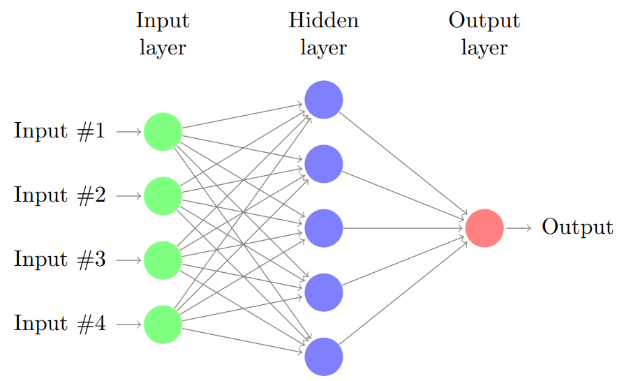
이러한 구조의 perceptron을 MLP(Multi Layer Perceptron)이라고 한다. MLP란 input layer와 output layer 사이에 hidden layers가 추가된 구조의 perceptrons를 의미한다.(참고로 하나의 hidden layer를 사용하는 MLP의 경우 Vanilla Neural Networks라고도 부르기도 한다.)

당시에는 이러한 Multi layer perceptron의 weights 들을 학습시킬 수 있는 적절한 방법이 없었지만, 이후에 Back propagation이 제시되면서 Multi layer perceptron을 적합시킬 수 있게 된다.

Back propagation

MLP의 개념이 처음 제시되었을 때에는 layer의 수가 많아질 경우 final output을 각 intput feature variable에 대하여 미분한 값(Gradient)를 구하여 Weight을 update하는 일이 쉽지 않다고 생각하였다. 하지만 이후에 Back propagation의 개념이 도입되면서 이 문제는 해결되고, Neural networks를 적합시킬 수 있게 된다.

사실 Back propagation은 사실 새로운 개념이 아닌, 미분적분학에서 사용하는 chain rule 그 자체일 뿐이다. 다음 그림을 살펴보자.

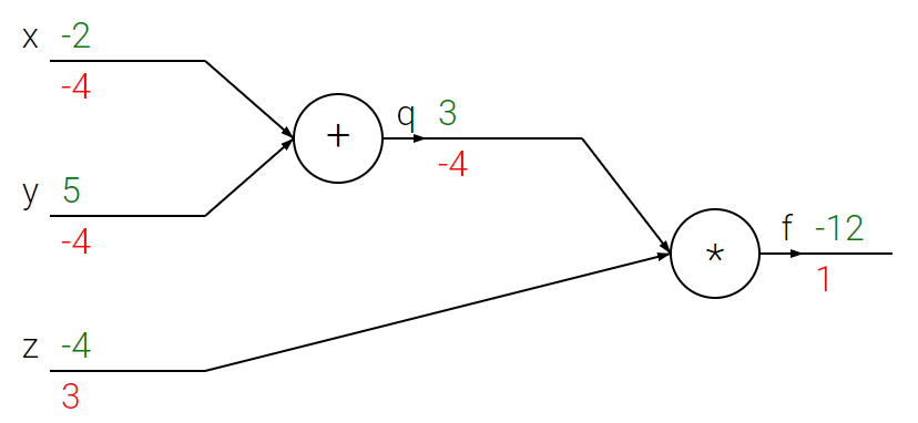
back propagation을 잘 설명해주는 그림이며, CS231n의 강의노트 Lecture 4에서 가져온 자료이다.

Input variable로 $[x, y, z]$ = $[-2, 5, -4]$를 가지고 있으며, Computational graph는 위와 같다.

이 예시에서는 $x+y = q$를 구한 후에 $z$를 곱해주는 연산을 통하여 최종 output $f = q \cdot z = (x+y) \cdot z$를 계산하는 구조를 가지고 있다.

우리는 $\partial f \over \partial x$, $\partial f \over \partial y$, $\partial f \over \partial z$를 계산해내야만 $x, y, z$에 대한 weight을 update할 수 있다. 우리가 복잡한 연산 없이 간단하게 계산할 수 있는 정보를 정리해보면 다음과 같다.

하지만 우리는 추가적으로 ${\partial f \over \partial x}$와 ${\partial f \over \partial y}$를 알고 싶은 상황이다. 이 때 back propagation을 활용하면 ${\partial f \over \partial x}$와 ${\partial f \over \partial y}$를 쉽게 구할 수 있다.

${\partial f \over \partial x}$와 ${\partial f \over \partial y}$는 다음과 같이 chain rule을 활용하여 계산할 수 있다.

참고로 이러한 계산은 우리의 모델에 존재하는 모든 weights들에 대하여 초기 값을 1이라고 가정하여 계산한 것이라고 볼 수 있고, 그 이후에는 위와 같이 local gradients와 global gradients를 구하고 나면 우리는 weights를 gradient를 반영하여 update해줄 수 있게 된다.

Source code

import torch

# setting device
device = 'cuda' if torch.cuda.is_available() else 'cpu'

# for reproducibility
torch.manual_seed(777)
if device == 'cuda':
    torch.cuda.manual_seed_all(777)

# dataset
X = torch.FloatTensor([[0, 0], [0, 1], [1, 0], [1, 1]]).to(device)
Y = torch.FloatTensor([[0], [1], [1], [0]]).to(device)

# model
linear1 = torch.nn.Linear(2, 10, bias=True)
linear2 = torch.nn.Linear(10, 10, bias=True)
linear3 = torch.nn.Linear(10, 10, bias=True)
linear4 = torch.nn.Linear(10, 1, bias=True)
sigmoid = torch.nn.Sigmoid()
model = torch.nn.Sequential(linear1, sigmoid, linear2, sigmoid, linear3, sigmoid, linear4, sigmoid).to(device)

# define cost/loss & optimizer
criterion = torch.nn.BCELoss().to(device)
optimizer = torch.optim.Adam(model.parameters(), lr=0.1)

for step in range(4001):
    # Hypothesis
    hypothesis = model(X)

    # cost/loss function
    cost = criterion(hypothesis, Y)

    # updating weights
    optimizer.zero_grad()
    cost.backward()
    optimizer.step()

    if step % 100 == 0:
        print(step, cost.item())

3개의 hidden layer를 가진 Multi layer perceptron이다.

# Accuracy computation
# True if hypothesis>0.5 else False
with torch.no_grad():
    hypothesis = model(X)
    predicted = (hypothesis > 0.5).float()
    accuracy = (predicted == Y).float().mean()
    print('\nHypothesis: ', hypothesis.detach().cpu().numpy(), '\nCorrect: ', predicted.detach().cpu().numpy(), '\nAccuracy: ', accuracy.item())

Test 결과 100%의 정확도로 예측에 성공한 것을 확인할 수 있다.

Reference

CS231n, Stanford University School of Engineering

모두를 위한 딥러닝 시즌2

PyTorch로 시작하는 딥 러닝 입문

Example: Neural network