우선, 해당 포스트는 Stanford University School of Engineering의 CS231n 강의자료와 모두를 위한 딥러닝 시즌2의 자료를 기본으로 하여 정리한 내용임을 밝힙니다.
Sigmoid
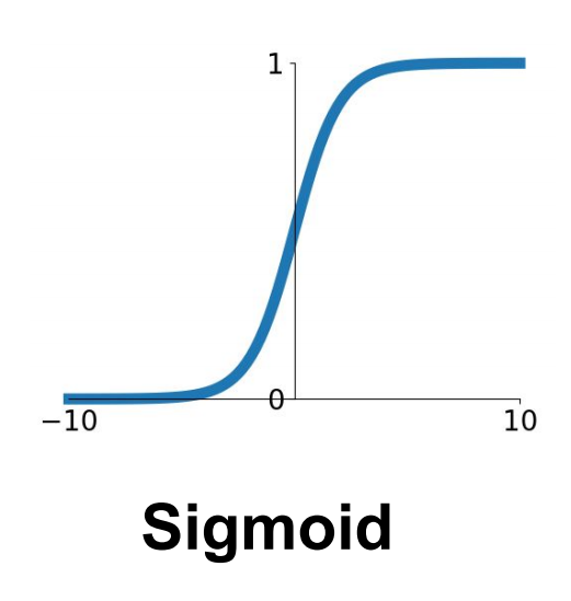
앞선 포스트에서 Activation 함수로써의 Sigmoid 함수에 대하여 세 가지 문제점을 살펴보았다. 그 중 Vanishing Gradient 와 Not zero centered 는 Neural Networks의 성능 저하에 큰 영향을 미치게 된다.
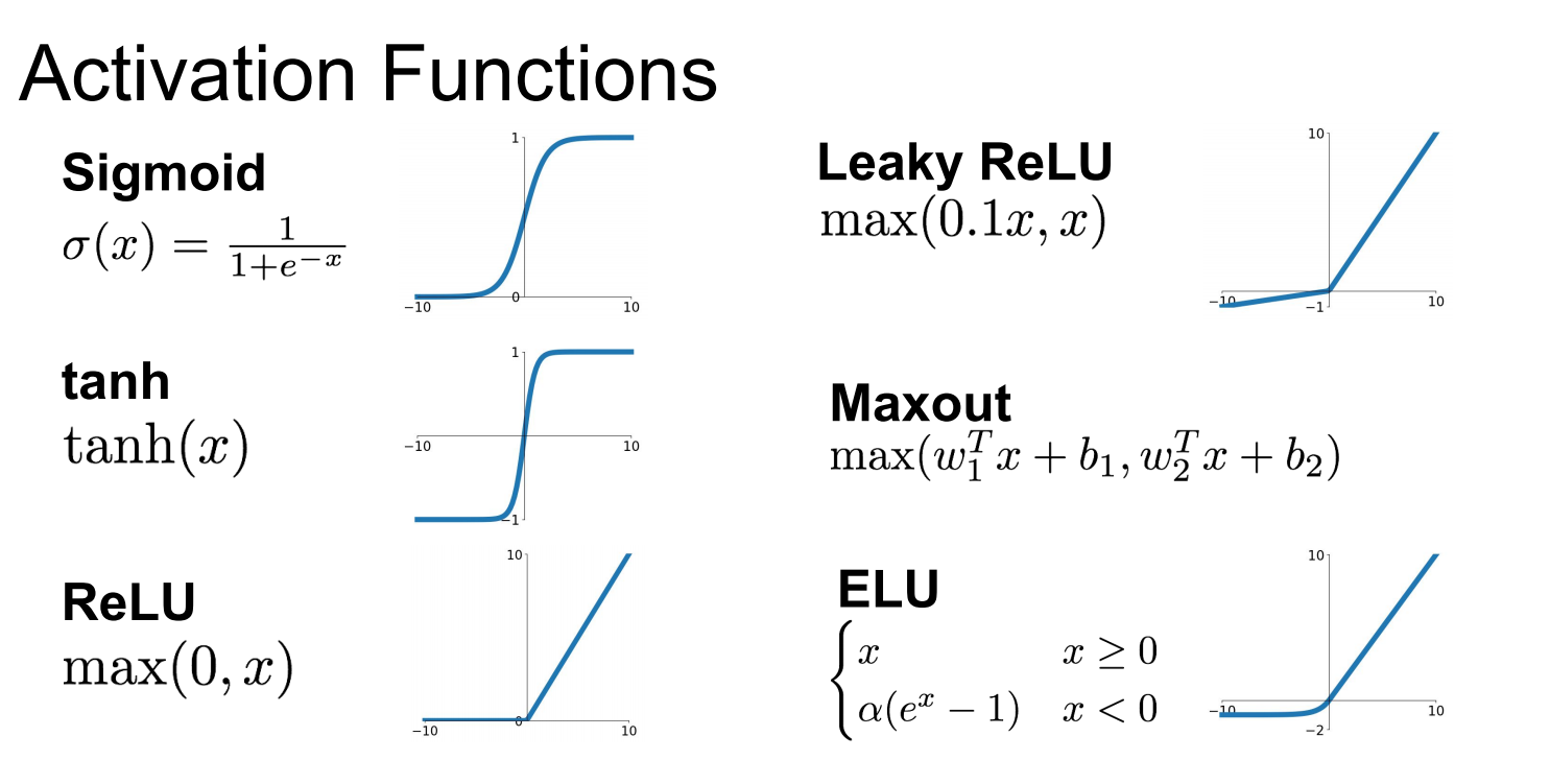
이러한 문제점을 해결하기 위하여 다양한 Activation 함수가 고안되었고, 이번 포스트에서는 tanh/ReLU/LeakyReLU/ELU/Maxout 함수에 대해 살펴보고자 한다.
tanh
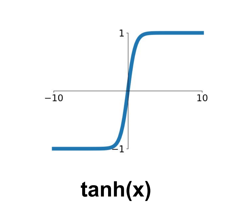
1991년, LeCun et al에 의해 제안된 Activation function이다.
0.5를 중심으로 하며, range[0,1]의 output 값을 가지는 Sigmoid 함수와는 달리, 0을 중심으로 range[-1,1]의 output 값을 가지는 함수이다.
Sigmoid 함수의 Not zero centered 의 단점을 보완하였다는 개선점이 있다. 하지만 너무 적거나 너무 큰 값에서는 Gradient가 0이되는 부분, 즉 Saturated Regime 이 여전히 존재한다는 문제점이 남아있다.
ReLU
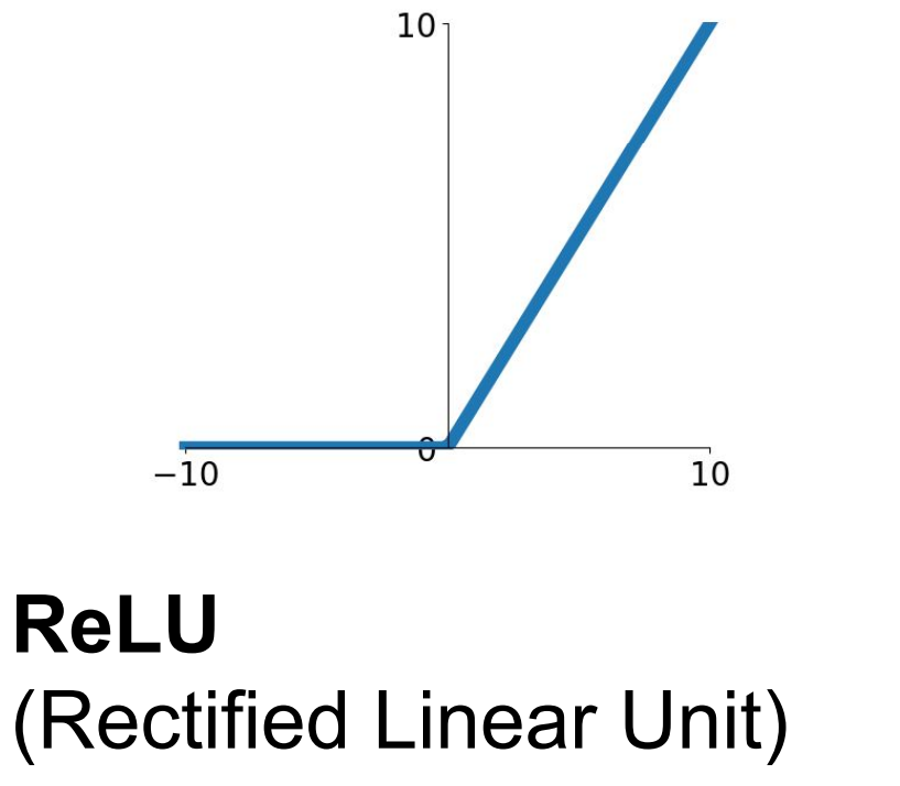
2012년, Krizhevsky et al에 의해 제안된 Activation function이다.
Sigmoid와 비교하였을 때, 물론 양수 부분에서만 Saturated Regime이 사라졌지만 Gradient Vanishing 문제가 어느정도 해결되었다는 것을 알 수 있다. 또한, exponential 함수 $exp$를 사용하지 않기 때문에 Computationally inefficient하다는 문제점도 해결되었다.
하지만 여전히 두 가지 큰 문제점이 남아있다. 첫 번째로 Sigmoid함수에서 존재하였던 Not zero-centered에 대한 문제를 해결하지 못하였으며, 두 번째로 음수 영역에서는 여전히 Gradient가 0이 되어 여전히 half of the regime에서 gradient를 “kill” 하고 있는 것이다.
LeakyReLU
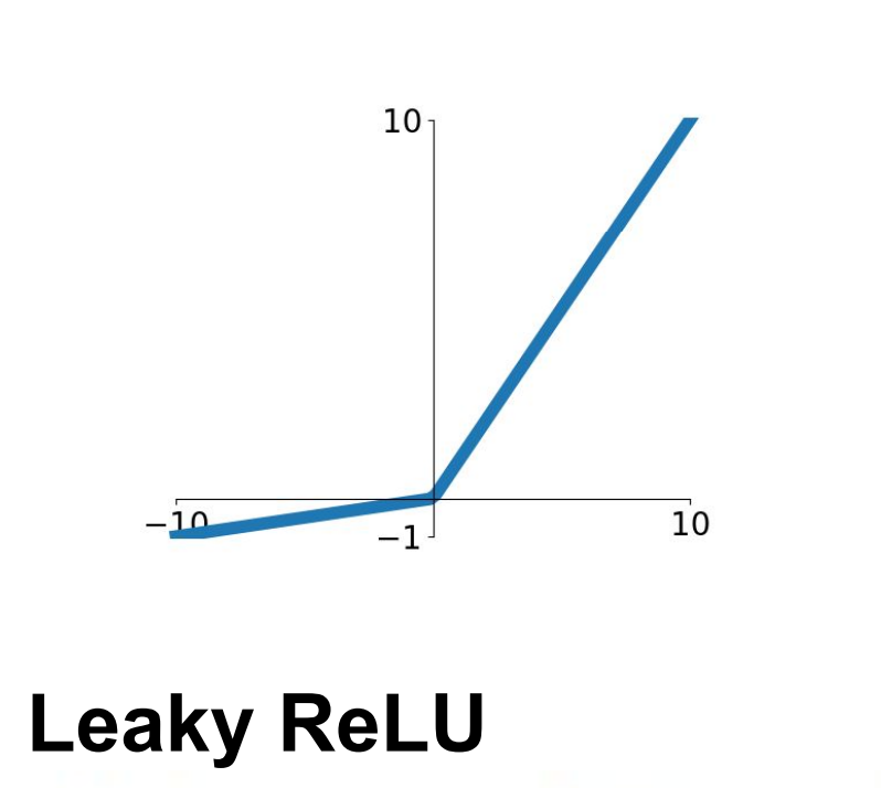
2013년, Mass et al과 2015년 He et al에 의해 제안된 Activation function이다.
ReLU 함수의 단점을 보완한 것이며, 무엇보다도 가장 중요한 것은 더 이상 음수 영역에서 Gradient가 0이 되어버리지 않는다는 장점이 있다. 또한, Computationally efficient하여 sigmoid 함수나 tanh 함수에 비하여 수렴 속도가 빠르다는 장점이 있다.
ELU
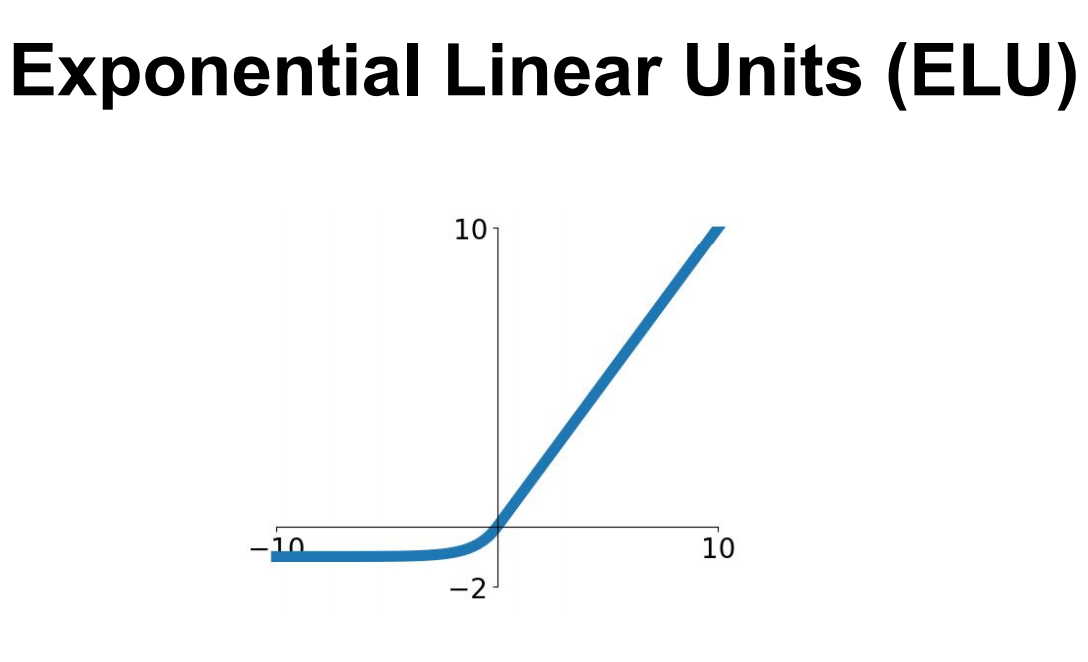
2015년, Clevert et al에 의해 제안된 Activation function이다.
\[\begin{align*} f(x) = \begin{cases} x\;\;\;\;\;\;\;\;\;\;\;\;\;\;\;\;\;\;\;\;\;\;if\;x>0\\\\ \alpha(exp(x)-1)\;\;\;if\;x\leq 0 \end{cases} \end{align*}\]이름에서 알 수 있듯이, ReLU의 좋은 점을 그대로 유지하면서 Zero-centered에 가깝게 변형한 함수이다.
단점으로는 exponential 함수를 사용하므로, Computationally Inefficient하다는 점이 있다.
Maxout
2013년, Goodfellow et al에 의해 제안된 Activation function이다.
\[max(w_1'x +b_1, w_2'x +b_2)\]앞서 살펴본 Activation functions들과는 조금은 다른 성격의 Activation 함수이다.
Saturated Regime이 없으며, Gradient가 0이 되어버리는 지점이 없다는 장점이 있다.
하지만 parameter의 수가 두 배가 되어버린다는 단점이 존재한다.
Summary
Stanford의 CS231n 강의에서는 다음과 같은 순서로 Activation function을 시도해볼 것을 권한다.
(1) ReLU를 사용하자.
(2) 성능이 만족스럽지 않다면, LeakyReLU, Maxout, ELU를 사용하라.
(3) 그래도 만족스럽지 않다면, tanh를 사용하라. 하지만 많은 기대는 하지말자.
(4) 그러나 Sigmoid는 사용하지 말라.
실무적으로는 ReLU를 가장 많이 사용하며, LeakyReLU/Maxout/ELU도 좋은 선택지가 될 수 있다.
Example
Softmax classifier를 활용한 MNIST classification에서 수정된 버전이다.
import torch
import torchvision.datasets as dsets
import torchvision.transforms as transforms
import random

# setting device
device = 'cuda' if torch.cuda.is_available() else 'cpu'

# for reproducibility
random.seed(111)
torch.manual_seed(777)
if device == 'cuda':
    torch.cuda.manual_seed_all(777)

# parameters
learning_rate = 0.001
training_epochs = 15
batch_size = 100

# MNIST dataset
mnist_train = dsets.MNIST(root='MNIST_data/',
                          train=True,
                          transform=transforms.ToTensor(),
                          download=True)

mnist_test = dsets.MNIST(root='MNIST_data/',
                         train=False,
                         transform=transforms.ToTensor(),
                         download=True)

# dataset loader
data_loader = torch.utils.data.DataLoader(dataset=mnist_train,
                                          batch_size=batch_size,
                                          shuffle=True,
                                          drop_last=True)

# nn layers
linear1 = torch.nn.Linear(784, 256, bias=True)
linear2 = torch.nn.Linear(256, 256, bias=True)
linear3 = torch.nn.Linear(256, 10, bias=True)
relu = torch.nn.ReLU()
# Initialization
torch.nn.init.normal_(linear1.weight)
torch.nn.init.normal_(linear2.weight)
torch.nn.init.normal_(linear3.weight)
# model
model = torch.nn.Sequential(linear1, relu, linear2, relu, linear3).to(device)

# define cost/loss & optimizer
criterion = torch.nn.CrossEntropyLoss().to(device)    # Softmax is internally computed.
optimizer = torch.optim.Adam(model.parameters(), lr=learning_rate)

total_batch = len(data_loader)
for epoch in range(training_epochs):
    avg_cost = 0

    for X, Y in data_loader:
        # reshape input image into [batch_size by 784]
        # label is not one-hot encoded
        X = X.view(-1, 28 * 28).to(device)
        Y = Y.to(device)

        optimizer.zero_grad()
        hypothesis = model(X)
        cost = criterion(hypothesis, Y)
        cost.backward()
        optimizer.step()

        avg_cost += cost / total_batch

    print('Epoch:', '%04d' % (epoch + 1), 'cost =', '{:.9f}'.format(avg_cost))
print('Learning finished')
softmax classifier에서는 하나의 layer를 사용하였으나, 이번 예제에서는 hidden layer 2개를 더 추가해 주었다.
또한 Sigmoid 함수 대신, ReLU함수를 Activation function으로 사용해 주었다. 마지막 layer(layer3)의 뒷단에 ReLU함수를 적용해주지 않은 이유는 CrossEntropyLoss를 사용하였기 때문이다.(Pytorch의 경우, CrossEntropyLoss 내부에 Sigmoid 함수가 들어가 있다.)
# Test the model using test sets
with torch.no_grad():
    X_test = mnist_test.test_data.view(-1, 28 * 28).float().to(device)
    Y_test = mnist_test.test_labels.to(device)

    prediction = model(X_test)
    correct_prediction = torch.argmax(prediction, 1) == Y_test
    accuracy = correct_prediction.float().mean()
    print('Accuracy:', accuracy.item())

    # Get one and predict
    r = random.randint(0, len(mnist_test) - 1)
    X_single_data = mnist_test.test_data[r:r + 1].view(-1, 28 * 28).float().to(device)
    Y_single_data = mnist_test.test_labels[r:r + 1].to(device)

    print('Label: ', Y_single_data.item())
    single_prediction = model(X_single_data)
    print('Prediction: ', torch.argmax(single_prediction, 1).item())
단순한 Softmax Classifier의 경우 86.9% 정도의 Accuracy를 보여주었었는데, 이번 예제의 Neural Networks(3 layers, ReLu activations)에서는 94.7%의 Accuracy를 보여준다.
Reference
CS231n, Stanford University School of Engineering