Regularization/Dropout

우선, 해당 포스트는 Stanford University School of Engineering의 CS231n 강의자료와 모두를 위한 딥러닝 시즌2의 자료를 기본으로 하여 정리한 내용임을 밝힙니다.

Overfitting

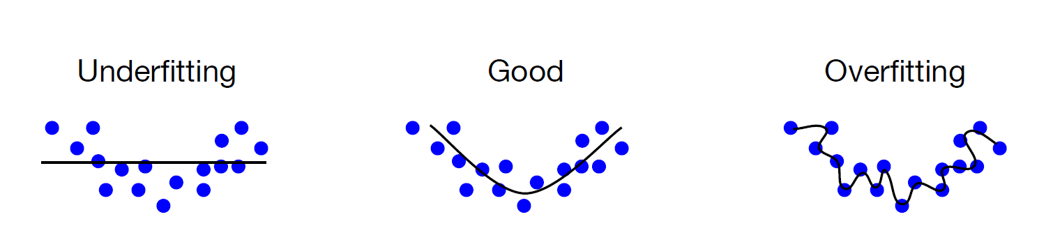
오버피팅(overfitting)이란 training data 를 과하게 학습하는 것을 뜻한다. training data를 과하게 학습하는 것이 어떤 문제가 될까?

일반적으로 Training data는 실제 데이터의 부분 집합이므로 training data 에 대해서는 Error가 감소 하지만, Test data 에 대해서는 Error가 증가 하게 된다.

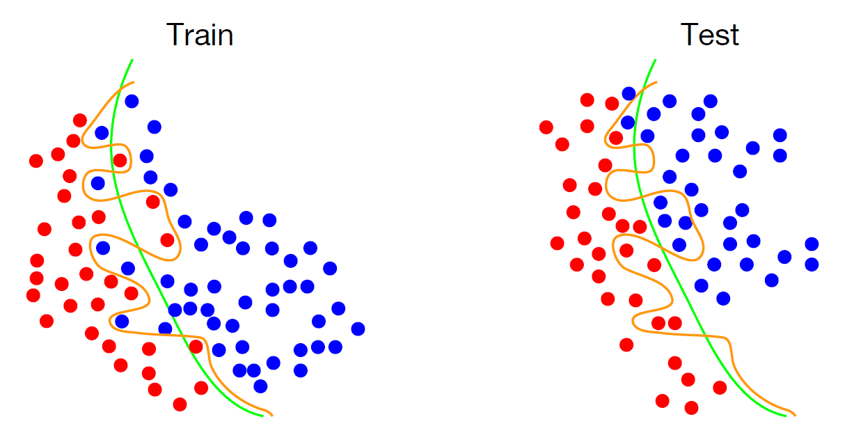
위 예시의 overfitting된 모델에서도, Test dataset에 대하여 Error가 꽤 증가하는 것을 확인할 수 있다.

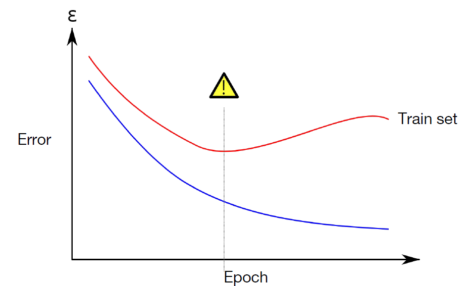
과적합을 할수록 Training dataset에 대한 Error는 계속 줄어들겠지만, Validation set에 대한 Error는 어느 순간부터 증가하기 마련이다. 이 때 우리는 모델이 Overfitting 되어 있다고 한다.

Regularization

Overfitting을 해결하기 위해 Regularization을 도입하게 되며, Deep learning에서 많이 사용되는 Regularization 방법에는 loss에 새로운 Regularization term을 더해주거나, Drop out을 사용하는 등의 여러 방법이 존재한다. 이번 포스트에서는 loss에 새로운 term을 더해주는 방식과 Drop out에 대해 살펴보도록 하겠다.

Add term to loss

\[L = {\frac 1 N} \sum_{i=1}^N \sum_{i \neq y_i} max(0,f(x_i;W)_ j -f(x_i;W)_ {y_i}+1)+\lambda R(W)\]

위와 같이 Loss에 Regularization term을 추가해주는 방법으로 Overfitting을 해결할 수 있다.

Regularization term $R(W)$의 대표적인 예시로는 다음과 같은 $L1$ Regularization, $L2$ Regularization, Elastic net$(L1+L2)$등이 있다.

\[\begin{align*} \text{L2 Regularization: } R(W) &= \sum_k \sum_l W_{k,l}^2\\ \text{L1 Regularization: } R(W) &= \sum_k \sum_l \vert W_{k,l} \vert \\ \text{Elastic net(L1+L2): } R(W) &= \sum_k \sum_l \beta W_{k,l}^2 + \vert W_{k,l} \vert\\ \end{align*}\]

Dropout

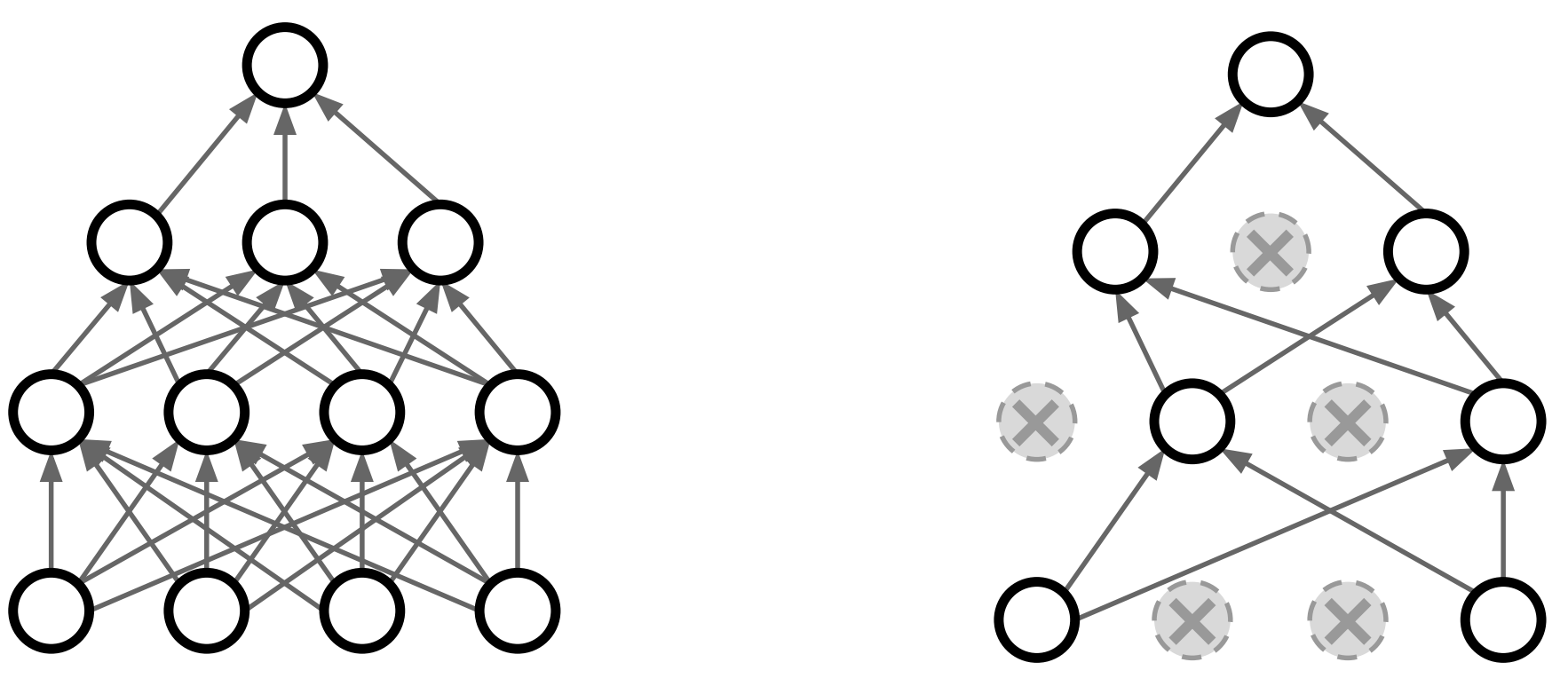
Dropout이란 Training시에 일정 비율의 Neuron만 사용하고, 나머지 Neuron에 해당하는 Weight은 update하지 않는 방법이다. 물론 매 step마다 사용하지 않는 Neuron을 바꿔가며 training시킨다. Default 값으로는 0.5를 많이 사용한다.

이렇게 Dropout을 통하여 각기 다른 Neuron들로 이루어진 각 step마다의 모델은 하나의 같은 모델 내에서 마치 다른 모델들인 것처럼 Training되게 된다. 즉, Dropout으로 하나의 모델 안에서 여러 모델을 앙상블하는 효과를 얻을 수 있다.

Dropout을 사용하면 Training time이 길어지는 단점이 존재하지만, 모델의 성능 향상을 위해 상당히 자주 사용되는 방법이다.

Example: Dropout

import torch
import torchvision.datasets as dsets
import torchvision.transforms as transforms
import random

# setting device
device = 'cuda' if torch.cuda.is_available() else 'cpu'

# for reproducibility
random.seed(777)
torch.manual_seed(777)
if device == 'cuda':
    torch.cuda.manual_seed_all(777)

# parameters
learning_rate = 0.001
training_epochs = 15
batch_size = 100
drop_prob = 0.3

# MNIST dataset
mnist_train = dsets.MNIST(root='MNIST_data/',
                          train=True,
                          transform=transforms.ToTensor(),
                          download=True)

mnist_test = dsets.MNIST(root='MNIST_data/',
                         train=False,
                         transform=transforms.ToTensor(),
                         download=True)

# dataset loader
data_loader = torch.utils.data.DataLoader(dataset=mnist_train,
                                          batch_size=batch_size,
                                          shuffle=True,
                                          drop_last=True)

# nn layers
linear1 = torch.nn.Linear(784, 512, bias=True)
linear2 = torch.nn.Linear(512, 512, bias=True)
linear3 = torch.nn.Linear(512, 512, bias=True)
linear4 = torch.nn.Linear(512, 512, bias=True)
linear5 = torch.nn.Linear(512, 10, bias=True)
relu = torch.nn.ReLU()
dropout = torch.nn.Dropout(p=drop_prob)

# xavier initialization
torch.nn.init.xavier_uniform_(linear1.weight)
torch.nn.init.xavier_uniform_(linear2.weight)
torch.nn.init.xavier_uniform_(linear3.weight)
torch.nn.init.xavier_uniform_(linear4.weight)
torch.nn.init.xavier_uniform_(linear5.weight)

# model
model = torch.nn.Sequential(linear1, relu, dropout,
                            linear2, relu, dropout,
                            linear3, relu, dropout,
                            linear4, relu, dropout,
                            linear5).to(device)

# define cost/loss & optimizer
criterion = torch.nn.CrossEntropyLoss().to(device)    # Softmax is internally computed.
optimizer = torch.optim.Adam(model.parameters(), lr=learning_rate)

total_batch = len(data_loader)
model.train()    # set the model to train mode (dropout=True)
for epoch in range(training_epochs):
    avg_cost = 0

    for X, Y in data_loader:
        # reshape input image into [batch_size by 784]
        # label is not one-hot encoded
        X = X.view(-1, 28 * 28).to(device)
        Y = Y.to(device)

        optimizer.zero_grad()
        hypothesis = model(X)
        cost = criterion(hypothesis, Y)
        cost.backward()
        optimizer.step()

        avg_cost += cost / total_batch

    print('Epoch:', '%04d' % (epoch + 1), 'cost =', '{:.9f}'.format(avg_cost))

print('Learning finished')

# Test model and check accuracy
with torch.no_grad():
    model.eval()    # set the model to evaluation mode (dropout=False)

    # Test the model using test sets
    X_test = mnist_test.data.view(-1, 28 * 28).float().to(device)
    Y_test = mnist_test.targets.to(device)

    prediction = model(X_test)
    correct_prediction = torch.argmax(prediction, 1) == Y_test
    accuracy = correct_prediction.float().mean()
    print('Accuracy:', accuracy.item())

    # Get one and predict
    r = random.randint(0, len(mnist_test) - 1)
    X_single_data = mnist_test.data[r:r + 1].view(-1, 28 * 28).float().to(device)
    Y_single_data = mnist_test.targets[r:r + 1].to(device)

    print('Label: ', Y_single_data.item())
    single_prediction = model(X_single_data)
    print('Prediction: ', torch.argmax(single_prediction, 1).item())

Reference

CS231n, Stanford University School of Engineering

모두를 위한 딥러닝 시즌2