우선, 해당 포스트는 Stanford University School of Engineering의 CS231n 강의자료와 모두를 위한 딥러닝 시즌2의 자료를 기본으로 하여 정리한 내용임을 밝힙니다.
Convolutional Neural Networks
앞서 우리는 Softmax Classifier, Neural Networks(MLP) 등의 모델을 통하여 MNIST dataset의 classification 문제를 풀어보았다. 지금까지는 $28 \times 28$ 크기의 이미지를 다루기 위하여 $28 \times 28$ 행렬을 $1 \times 784$ 형태의 벡터로 reshape 해주어 input으로 사용했다. 하지만 이러한 방식은 데이터의 공간 정보 를 유실시키는 결과를 가져오고, 이로인하여 모델의 성능은 저하될 수밖에 없다.
반면, CNN에서는 Convolution layer 을 도입하여 이 문제를 해결하게 된다. CNN은 $28 \times 28$을 일렬로 펼친 형태의 벡터로 reshape해주지 않고, $28 \times 28$의 이미지 데이터를 그대로 사용한다.
그렇다면 Convolution layer 가 무엇인지에 대하여 조금 더 자세히 살펴보도록 하자.
Convolution Layer
vdumoulin github에 Convolution layer의 연산 방식을 잘 나타낸 그림이 있어서 가져와 보았다.
위 그림은 $4 \times 4$의 input data에 $3 \times 3$의 filter를 적용하여 $2 \times 2$의 output을 구하는 과정을 보여준다. output 행렬의 각 element를 계산하는 방식은 아래 예시에서 조금 더 자세히 살펴보도록 하겠다.
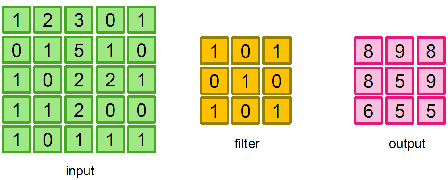
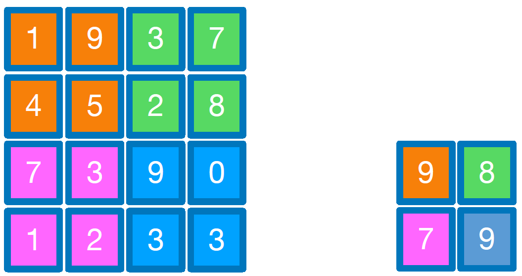
간단한 설명을 위하여 $5 \times 5$의 input data가 있다고 하자.(초록색)
Convolution layer는 filter 행렬을 사용하여 연산하고(주황색), output 행렬을 구해낸다.(분홍색)
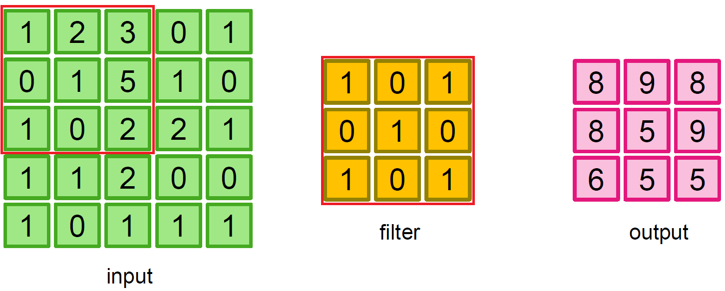
output 행렬의 1행 1열의 값을 구하는 과정은 위와 같이 element-wise multiplication 연산을 계산하여 최종적으로 합해준다. 나머지 elements에 대해서도 똑같은 방식으로 연산해주면 최종적인 output 행렬을 구할 수 있다.
이러한 방식으로 Filter를 사용하여 연산해주는 layer를 Convolution Layer라고 한다.
이번에는 또 다른 예시로 MNIST 데이터를 통해 실제 데이터에서 연산되는 과정을 한 번 살펴보도록 하자.
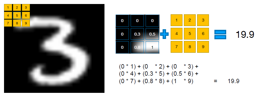
$28 \times 28$의 input data에 $3 \times 3$의 filter를 적용하여 계산하여 output 행렬의 1행 1열의 성분을 계산하는 과정을 나타낸 것이다. 행렬의 나머지 성분들 또한 마찬가지로 element-wise multiplication을 해준 후, 이를 더해주는 과정을 거쳐 계산이 이루어진다.
Convolution Layer: stride
Convolution layer에는 다양한 옵션을 줄 수 있는데, 그 중 하나가 Stride 이다.
Stride는 filter를 한 번에 얼마나 이동시킬 것인가를 의미한다. 위 예시에서는 filter가 두 칸씩 이동하고 있으므로, Stride=2 로 설정해준 것이다. 만약 Stride를 따로 설정해주지 않을 경우에는 Stride=1 이 기본적인 default 값으로 사용된다.
Convolution Layer: zero padding
zero padding 은 input의 size를 유지해주면서, edge의 정보를 잃지 않게 하기위하여 사용하는 방법이다. 위 예시와 같이 data의 edge 바깥 부분을 0으로 채워주는 방법을 zero padding이라고 한다. 위와 같이 0으로 두 겹을 쌓아줄 경우 padding=2 옵션이며, 따로 설정해주지 않을 경우에는 padding=0 이 default 옵션으로 사용된다.
Convolution Layer: output size
결과적으로, Convolution Layer를 거쳐 나오는 output의 shape은 다음과 같다.
\[\text{output size } = {\frac {\text{input size} - \text{filter size} + (2 \times \text{padding})} {\text{stride}}} + 1\]
torch.nn.Conv2d()
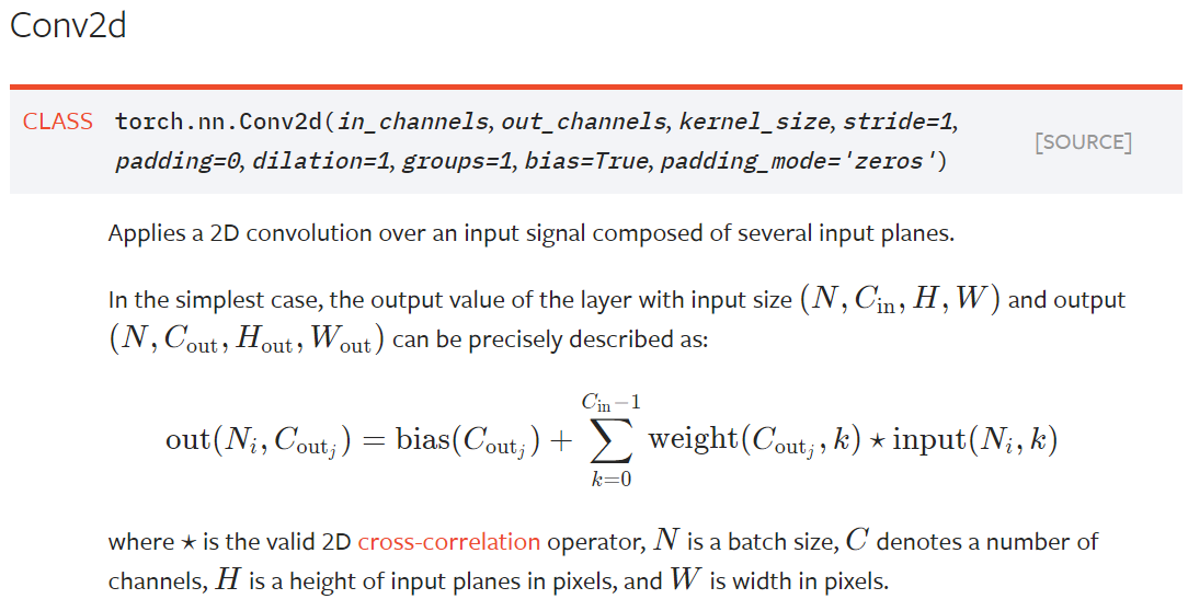
Pytorch 공식 홈페이지의 Documentation에 나와있는 Convolution layer를 구현한 함수이다.
Pytorch의 torch.nn.Conv2d()의 경우, input data로 사용하는 데이터는 torch.Tensor 여야 하며, 다음과 같은 shape을 가지고 있어야 한다.
Pooling layer
CNN에서 사용되는 또 하나의 layer가 있는데, 바로 Pooling layer이다. Pooling layer는 Down sampling을 위해 사용되는데, 대표적인 예시로 Max pooling이나 Average Pooling이 있다.
Max pooling의 경우, filter 안에 들어오는 elements 중에서 가장 큰 값을 선택하여 output 행렬의 element로 사용하는 방식이다. 위 그림은 Max pooling의 간단한 예시이다.
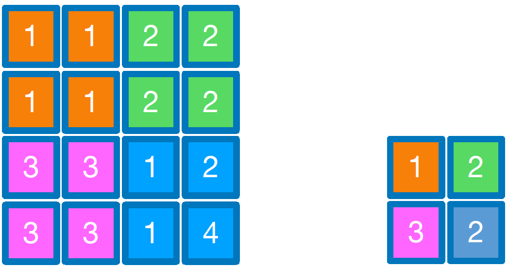
반면, Average pooling의 경우, filter 안에 들어오는 elements에 대하여 평균 값을 구하여 output 행렬의 element로 사용하는 방식이다. 위 그림은 Average pooling의 예시이다.
torch.nn.MaxPool2d()
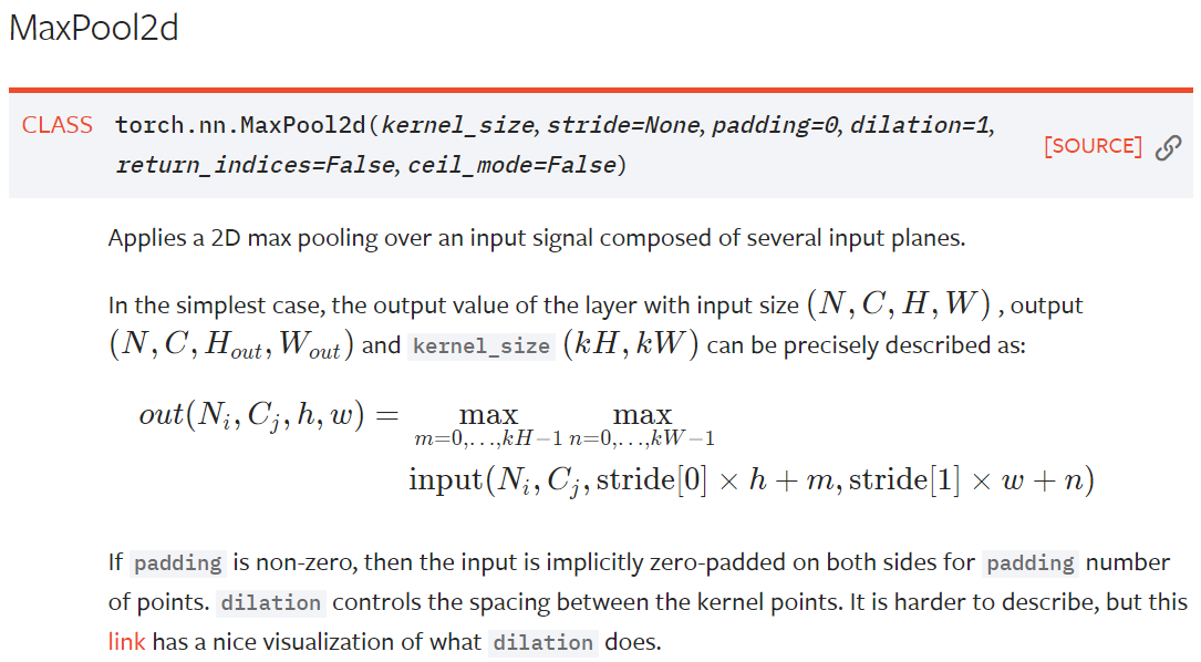
Pytorch 공식 홈페이지의 Documentation에 나와있는 Max pooling layer를 구현한 함수이다.
torch.nn.AvgPool2d()
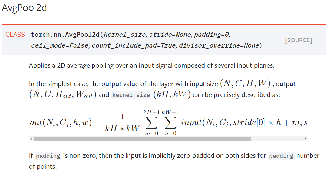
Pytorch 공식 홈페이지의 Documentation에 나와있는 Average pooling layer를 구현한 함수이다.
Example
CNN을 활용한 MNIST classification 문제를 풀어보자.
우리가 사용할 모델의 구조는 다음과 같다.
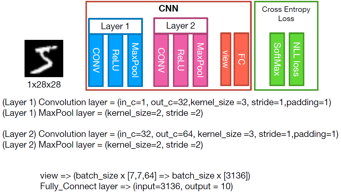
위 구조의 CNN을 Pytorch로 구현해보면 다음과 같다.
import torch
import torchvision.datasets as dsets
import torchvision.transforms as transforms
import torch.nn.init

# setting device
device = 'cuda' if torch.cuda.is_available() else 'cpu'

# for reproducibility
torch.manual_seed(777)
if device == 'cuda':
    torch.cuda.manual_seed_all(777)

# parameters
learning_rate = 0.001
training_epochs = 15
batch_size = 100

# MNIST dataset
mnist_train = dsets.MNIST(root='MNIST_data/',
                          train=True,
                          transform=transforms.ToTensor(),
                          download=True)

mnist_test = dsets.MNIST(root='MNIST_data/',
                         train=False,
                         transform=transforms.ToTensor(),
                         download=True)

# dataset loader
data_loader = torch.utils.data.DataLoader(dataset=mnist_train,
                                          batch_size=batch_size,
                                          shuffle=True,
                                          drop_last=True)

# CNN Model (2 conv layers)
class CNN(torch.nn.Module):

    def __init__(self):
        super(CNN, self).__init__()
        # L1 ImgIn shape=(?, 28, 28, 1)
        #    Conv     -> (?, 28, 28, 32)
        #    Pool     -> (?, 14, 14, 32)
        self.layer1 = torch.nn.Sequential(
            torch.nn.Conv2d(1, 32, kernel_size=3, stride=1, padding=1),
            torch.nn.ReLU(),
            torch.nn.MaxPool2d(kernel_size=2, stride=2))
        # L2 ImgIn shape=(?, 14, 14, 32)
        #    Conv      ->(?, 14, 14, 64)
        #    Pool      ->(?, 7, 7, 64)
        self.layer2 = torch.nn.Sequential(
            torch.nn.Conv2d(32, 64, kernel_size=3, stride=1, padding=1),
            torch.nn.ReLU(),
            torch.nn.MaxPool2d(kernel_size=2, stride=2))
        # Final FC 7x7x64 inputs -> 10 outputs
        self.fc = torch.nn.Linear(7 * 7 * 64, 10, bias=True)
        torch.nn.init.xavier_uniform_(self.fc.weight)

    def forward(self, x):
        out = self.layer1(x)
        out = self.layer2(out)
        out = out.view(out.size(0), -1)   # Flatten them for FC
        out = self.fc(out)
        return out

# instantiate CNN model
model = CNN().to(device)

# define cost/loss & optimizer
criterion = torch.nn.CrossEntropyLoss().to(device)    # Softmax is internally computed.
optimizer = torch.optim.Adam(model.parameters(), lr=learning_rate)

# train my model
total_batch = len(data_loader)
print('Learning started. It takes sometime.')
for epoch in range(training_epochs):
    avg_cost = 0

    for X, Y in data_loader:
        # image is already size of (28x28), no reshape
        # label is not one-hot encoded
        X = X.to(device)
        Y = Y.to(device)

        optimizer.zero_grad()
        hypothesis = model(X)
        cost = criterion(hypothesis, Y)
        cost.backward()
        optimizer.step()

        avg_cost += cost / total_batch

    print('[Epoch: {:>4}] cost = {:>.9}'.format(epoch + 1, avg_cost))
print('Learning Finished!')
# Test model and check accuracy
with torch.no_grad():
    X_test = mnist_test.data.view(len(mnist_test), 1, 28, 28).float().to(device)
    Y_test = mnist_test.targets.to(device)

    prediction = model(X_test)
    correct_prediction = torch.argmax(prediction, 1) == Y_test
    accuracy = correct_prediction.float().mean()
    print('Accuracy:', accuracy.item())
98.6% 정도의 정확도로, 이전의 포스트에서 시도해 보았던 여러 모델 중에서 가장 높은 정확도를 보이는 것을 확인할 수 있다.
Reference
CS231n, Stanford University School of Engineering