CNN Architecture(1)-LeNet

우선, 해당 포스트는 Stanford University School of Engineering의 CS231n 강의자료를 기본으로 하여 정리한 내용임을 밝힙니다.

CNN Architectures

이번 포스트 부터는 역사적으로 깊은 의미를 가지거나, ILSVRC에서 좋은 성적을 보여주었던 CNN Architecture들을 살펴보도록 할 것이다.

LeNet(1998)

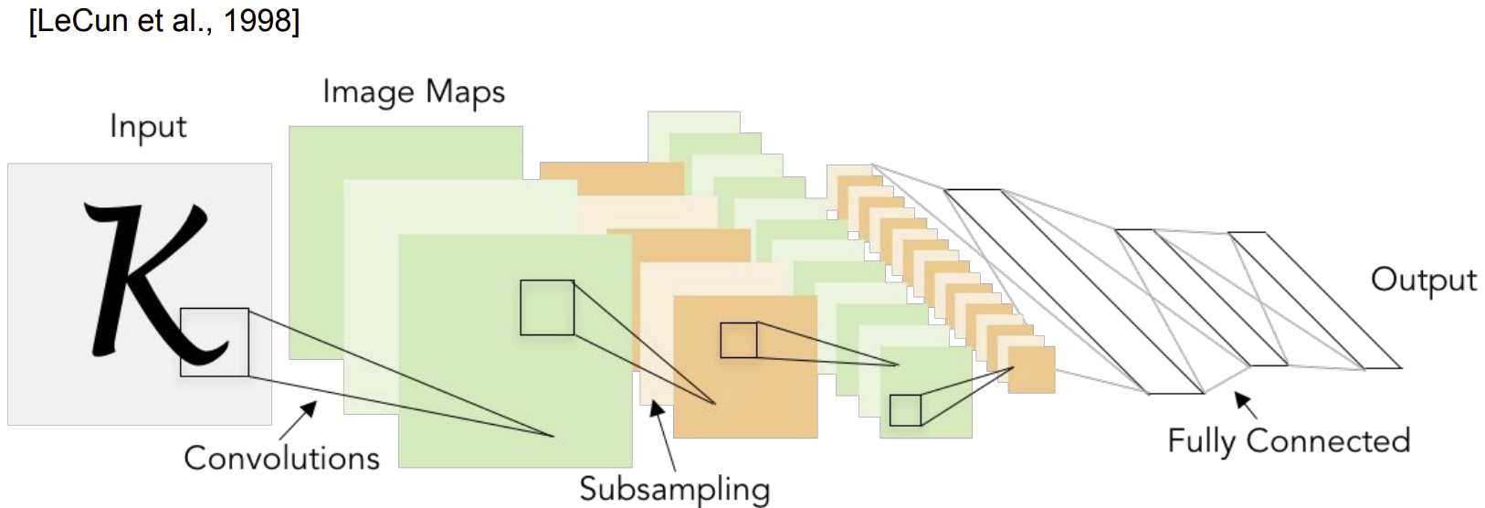
paper: LeCun et al.(1998), GradientBased Learning Applied to Document Recognition

우리가 알고 있는 CNN(Convolutional Neural Networks)을 가장 처음 도입한 사람은 프랑스의 얀 르쿤(Yann LeCun)이며, 현재는 Facebook의 Vice President, Chief AI Scientist를 맡고 있다.

LeNet의 경우 LeNet-1부터 LeNet-5까지 다양한 버전으로 존재한다. LeNet-1의 경우 1990년에 발표되었으며, 비교적 가장 최신의 LeNet에 해당하는 LeNet-5의 초기 모델로 볼 수 있다.

LeNet-1

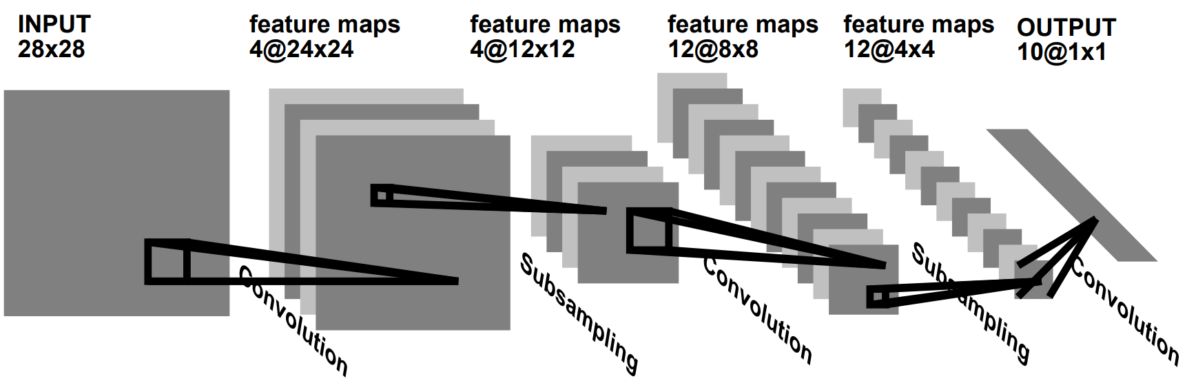
LeNet-1의 구조를 모델의 앞단부터 살펴보면 다음과 같다.

• 28×28 input image

• Four 24×24 feature maps convolutional layer (5×5 size)

• Average Pooling layers (2×2 size)

• Twelve 8×8 feature maps convolutional layer (5×5 size)

• Average Pooling layers (2×2 size)

• Directly fully connected to the output

이제 각 Layer의 ouput size를 차근차근 확인해보도록 하자.

우선, input image의 size는 $28 \times 28$이다.

첫 번째 Layer(Convolutional layer)는 4개의 $5 \times 5$ size filter를 사용하게 된다. 따라서 output의 경우 $24 \times 24 \times 4$가 된다.

두 번째 Layer(Pooling layer)에서는 $2 \times 2$ size의 kernel을 사용하며, 따라서 output의 dimension은 $12 \times 12 \times 4$가 된다.

세 번재 Layer는 다시 Convolutional Layer이며, 12개의 $5 \times 5$ size filter를 사용한다. 따라서 ouput의 dimension은 $8 \times 8 \times 12$이 된다.

네 번째 Layer는 Pooling layer로써, $2 \times 2$ size의 kernel로 Average Pooling을 해준다. 따라서 output의 dimension은 $4 \times 4 \times 12$가 된다.

이제 마지막으로, Fully Connected Layer를 거쳐 최종적으로 $1 \times 1 \times 10$의 output을 뽑아낸다.

LeNet의 경우 $5 \times 5$ size의 filter를 사용하는 Convolutional Layer를 통하여 Local receptive field 개념을 적용하였고, 네트워크 내에서 이미지에 대해 같은 Kernel을 적용함으로써 Shared weight 개념을 적용하였다는 의의를 가진다. 또한, Average pooling을 통하여 sub sampling 개념을 도입하였다는 점에서 이후의 CNN의 발전에 큰 기여를 하였다고 할 수 있다.

LeNet-5

LeCun은 LeNet을 통하여 CNN의 성능이 MLP(Multi Layer Perceptron), 혹은 DNN(Deep Neural Networks)을 비롯한 다른 분류 알고리즘들에 비하여 매우 좋다는 것을 알리게 되었다.

LeNet-1 이후, 많은 연구 끝에 LeNet-1과 비슷한 구조의 다양한 모델이 연구되어 LeNet-5까지 이르게 된다.

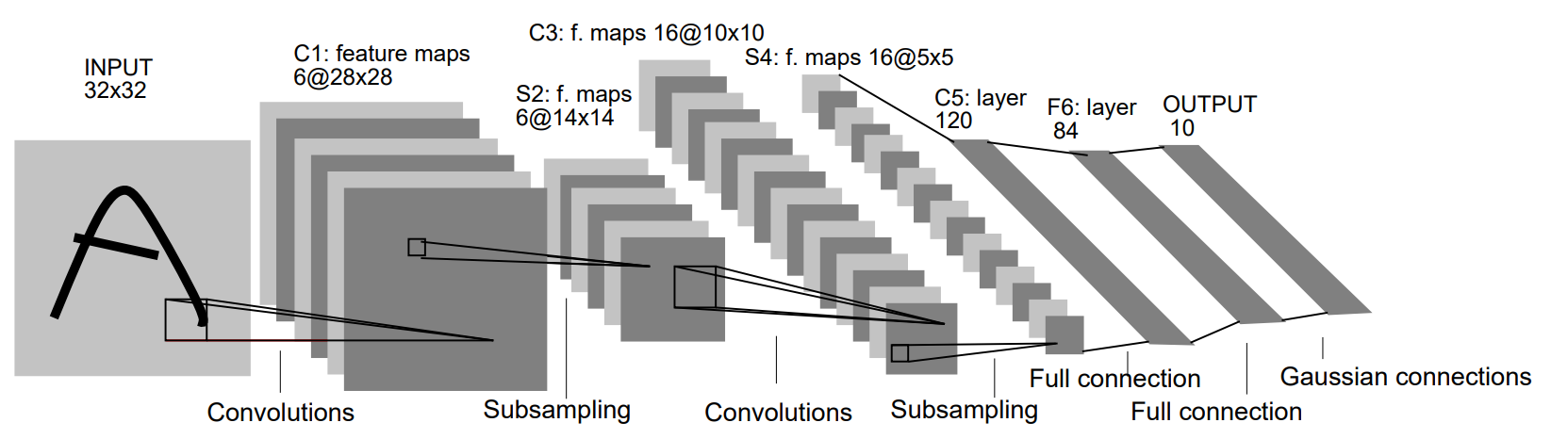
LeNet-5의 구조를 살펴보면 다음과 같다.

• 32×32 input image

• Six 28×28 feature maps convolutional layer (5×5 size)

• Average Pooling layers (2×2 size)

• Sixteen 10×10 feature maps convolutional layer (5×5 size)

• Average Pooling layers (2×2 size)

• Fully connected to 120 neurons

• Fully connected to 84 neurons

• Fully connected to 10 outputs

역시 각 Layer에서의 output size를 순서대로 살펴보도록 하자.

우선, input의 size는 $32 \times 32$이다.

첫 번째 Layer는 Convolutional Layer로써 6개의 $5 \times 5$ size filter를 사용한다. 따라서 output의 size는 $28 \times 28 \times 6$이 된다.

두 번째 Layer는 Pooling Layer로써 $2 \times 2$ size의 kernel을 사용하고, 결과적으로 output의 dimension은 $14 \times 14 \times 6$이 된다.

세 번째 layer는 Convolutional Layer로써 16개의 $5 \times 5$ size filter를 사용한다. 따라서 output의 size는 $10 \times 10 \times 16$이 된다.

네 번째 layer에서는 $2 \times 2$ size의 kernel을 통하여 다시 average pooling을 해주어 $5 \times 5 \times 16$의 output을 만들어낸다.

다섯 번째 layer는 FC Layer(Fully Connected Layer)로써 $1 \times 1 \times 120$ size의 output을 만들어낸다.

그에 이어 여섯 번째도 FC Layer로써 $1 \times 1 \times 84$의 output을 만들어낸다.

마지막 FC Layer에서는 최종적인 class의 수에 해당하는 10에 맞추어 $1 \times 1 \times 10$ size의 vector로 만들어준다.

Output size 계산

앞서 LeNet-1과 LeNet-5의 모든 Layer에서 output의 dimension을 계산해 보았다. 직접 새로운 데이터셋에서 새로운 모델을 만들어야 할 경우, dimension 계산을 잘 할수 있어야 모델을 잘 만들 수 있다. 따라서 Dimension 계산은 아주 중요한 작업이다.

각 Layer에서의 output size 계산은 다음과 같이 쉽게 할 수 있다.

(사실, LeNet과 같이 간단한 구조의 경우, 아래 식을 사용하지 않더라도 금방 계산할 수 있다. 하지만 복잡한 구조를 가진 CNN의 경우, 아래 식이 경우에 따라 큰 도움이 될 수도 있다.)

Convolutional layer

Pooling layer

Reference

LeCun et al.(1998), GradientBased Learning Applied to Document Recognition

Review: LeNet-1, LeNet-4, LeNet-5, Boosted LeNet-4 (Image Classification)